- 1 Overview
- 2 Environment Setup
- 3 A note on libraries
- 4 Data Import
- 5 Meta Data
- 6 Defining default
- 7 Removing variables deemed unfit for most modeling
- 8 A note on hypothesis generation vs. hypothesis confirmation
- 9 Exploratory Data Analysis
- 10 Correlation
- 11 Summary plots
- 12 Modeling
- 12.1 Model options
- 12.2 Imbalanced data
- 12.3 A note on modeling libraries
- 12.4 Data preparation for modeling
- 12.5 Logistic regression
- 12.6 Model evaluation illustration
- 12.7 Variable selection
- 12.8 A more complex logistic model with caret
- 12.9 A note on computational efficiency (parallelization via cluster)
- 12.10 A note on tuning parameters in caret
- 12.11 Trees
- 13 Further Resources
1 Overview
A case study of machine learning / modeling in R with credit default data. Data is taken from Kaggle Lending Club Loan Data but is also available publicly at Lending Club Statistics Page. We illustrate the complete workflow from data ingestion, over data wrangling/transformation to exploratory data analysis and finally modeling approaches. Along the way will be helpful discussions on side topics such as training strategy, computational efficiency, R intricacies, and more. Note that the focus is more on methods in R rather than statistical rigour. This is meant to be a reference for an end-to-end data science workflow rather than a serious attempt to achieve best model performance.
1.1 Kaggle Data Description
The files contain complete loan data for all loans issued through 2007-2015, including the current loan status (Current, Late, Fully Paid, etc.) and latest payment information. The file containing loan data through the “present” contains complete loan data for all loans issued through the previous completed calendar quarter. Additional features include credit scores, number of finance inquiries, address including zip codes, and state, and collections among others. The file is a matrix of about 890 thousand observations and 75 variables. A data dictionary is provided in a separate file.
2 Environment Setup
2.1 Libraries
This will automatically install any missing libraries. Make sure to have proper proxy settings. You do not necessarily need to have all of them but only those needed for respective sections (which will be indicated).
# define used libraries
libraries_used <-
  c("lazyeval", "readr","plyr" ,"dplyr", "readxl", "ggplot2",
    "funModeling", "scales", "tidyverse", "corrplot", "GGally", "caret",
    "rpart", "randomForest", "pROC", "gbm", "choroplethr", "choroplethrMaps",
    "microbenchmark", "doParallel", "e1071")

# check missing libraries
libraries_missing <-
  libraries_used[!(libraries_used %in% installed.packages()[,"Package"])]
# install missing libraries
if(length(libraries_missing)) install.packages(libraries_missing)
2.2 Session Info
sessionInfo()## R version 3.4.1 (2017-06-30)
## Platform: x86_64-w64-mingw32/x64 (64-bit)
## Running under: Windows 10 x64 (build 15063)
##
## Matrix products: default
##
## locale:
## [1] LC_COLLATE=English_United States.1252
## [2] LC_CTYPE=English_United States.1252
## [3] LC_MONETARY=English_United States.1252
## [4] LC_NUMERIC=C
## [5] LC_TIME=English_United States.1252
##
## attached base packages:
## [1] methods stats graphics grDevices utils datasets base
##
## loaded via a namespace (and not attached):
## [1] compiler_3.4.1 backports_1.1.0 bookdown_0.5 magrittr_1.5
## [5] rprojroot_1.2 tools_3.4.1 htmltools_0.3.6 yaml_2.1.14
## [9] Rcpp_0.12.12 stringi_1.1.5 rmarkdown_1.6 blogdown_0.1
## [13] knitr_1.17 stringr_1.2.0 digest_0.6.12 evaluate_0.10.13 A note on libraries
There are generally two ways to access functions from R packages (we use package and library interchangeably). Either via a direct access without loading the library, i.e. package::function() or by loading (attaching) the library into workspace (environment) and thus making all its functions available at once. The problem with the first option is that direct access sometimes can lead to issues (unexpected behavior/errors) and makes coding cumbersome. The problem with the second approach is a conflict of function (and other variables) names between two libraries (called masking). A third complication is that some functions require libraries to be loaded (e.g. some instances of caret::train()) and thus attach the library without being explicitly told. Again this may lead to masking of functions and if user is unaware this can lead to nasty problems (conceived bugs) down the road (sometimes libraries will issue a warning upon load, e.g. plyr when dplyr is already loaded). There is no golden way (at least we are not aware of it) and so we tend to do the following
- load major libraries that are used frequently into workspace but pay attention to load succession to avoid unwanted masking
- access rarely used functions directly (being aware that they work and don’t attach anything themselves)
- sometimes use direct access to a fucntion although its library is loaded (either to make clear which library is currently used or because we explicitly need a function that has been masked due to another loaded library)
We will load a few essential libraries here as they are used heavily. Other librraies may only be loaded in respective section. You can also try to follow the analysis without loading many librraies at the beginning but only when needed. Just be aware of the succession to avoid issues.
3.1 Library versions
Also note that often the version of the library used matters (it always matters but what we mean is, it makes a difference) and some libraries are developed more actively than others which may lead to issues. For example, note that library caret is using plyr while the tidyverse of which dplyr (successor of plyr) is part has some new concepts, e.g. the default data frame is a tibble::tibble(). It seems that caret has issues with tibbles, see e.g. “Wrong model type for classification” in regression problems in R-Caret.
library(plyr)
library(tidyverse)
## Loading tidyverse: ggplot2
## Loading tidyverse: tibble
## Loading tidyverse: tidyr
## Loading tidyverse: readr
## Loading tidyverse: purrr
## Loading tidyverse: dplyr## Conflicts with tidy packages ----------------------------------------------## arrange(): dplyr, plyr
## compact(): purrr, plyr
## count(): dplyr, plyr
## failwith(): dplyr, plyr
## filter(): dplyr, stats
## id(): dplyr, plyr
## lag(): dplyr, stats
## mutate(): dplyr, plyr
## rename(): dplyr, plyr
## summarise(): dplyr, plyr
## summarize(): dplyr, plyrlibrary(caret)## Loading required package: lattice##
## Attaching package: 'caret'## The following object is masked from 'package:purrr':
##
## lift4 Data Import
Refer to section Overview to see how the data may be acquired.
The loans data can be conveniently read via readr::read_csv(). Note that the function tries to determine the variable type by reading the first 1,000 rows which does not always guarantee correct import especially in cases of missing values at the begining of the file. Other packages treat imports differently, for example data.table::fread() takes a sample of 1,000 rows to determine column types (100 rows from 10 different points) which seems to get more robust results than readr::read_csv(). Both package functions allow the explicit definition of column classes, for readr::read_csv() it is parameter col_types and for data.table::fread() it is parameter colClasses. Alternatively, readr::read_csv() offers the parameter guess_max that allows increasing the number of rows being guessed similar to SAS import procedure parameter guessingrows. Naturally, import time increases if more rows are guessed. For details on readr including comparisons against Base R and data.table::fread() see readr.
path <- "D:/data/lending_club"
loans <- readr::read_csv(paste0(path, "./loan.csv"))
The meta data comes in an Excel file and needs to be parsed via a special library, in this case we use readxl.
library(readxl)
# Load the Excel workbook
excel_file = paste0("./LendingClubDataDictionary.xlsx")
# see available tabs
excel_sheets(paste0(path, excel_file))
## [1] "LoanStats" "browseNotes" "RejectStats"# Read in the first worksheet
meta_loan_stats = read_excel(paste0(path, excel_file), sheet = "LoanStats")
meta_browse_notes = read_excel(paste0(path, excel_file), sheet = "browseNotes")
meta_reject_stats = read_excel(paste0(path, excel_file), sheet = "RejectStats")5 Meta Data
Let’s have a look at the meta data in more detail. First, which variables are present in loan data set and what is their type. Then check meta data information and finally compare the two to see if anything is missing.
The usual approach may be to use base::str() function to get a summary of the data structure. However, it may be useful to quantify the “information power” of different metrics and dimensions by looking at the ratio of zeros and missing values to overall observations. This will not always reveal the truth (as there may be variables that are only populated if certain conditions apply) but it still gives some indication. The funModeling package offers the function funModeling::df_status() for that. It does not scale very well and has quite a few dependencies (so a direct call is preferred over a full library load) but it suits the purpose for this data. Unfortunately, it does not return the number of rows and columns. The data has 887379 observations (rows) and 74 variables (columns).
We will require the meta data at a later stage so we assign it to a variable. The function funModeling::df_status() has parameter print_results = TRUE set by default which means the data will be assigned and printed at the same time.
meta_loans <- funModeling::df_status(loans, print_results = FALSE)
knitr::kable(meta_loans)| variable | q_zeros | p_zeros | q_na | p_na | q_inf | p_inf | type | unique |
|---|---|---|---|---|---|---|---|---|
| id | 0 | 0.00 | 0 | 0.00 | 0 | 0 | integer | 887379 |
| member_id | 0 | 0.00 | 0 | 0.00 | 0 | 0 | integer | 887379 |
| loan_amnt | 0 | 0.00 | 0 | 0.00 | 0 | 0 | numeric | 1372 |
| funded_amnt | 0 | 0.00 | 0 | 0.00 | 0 | 0 | numeric | 1372 |
| funded_amnt_inv | 233 | 0.03 | 0 | 0.00 | 0 | 0 | numeric | 9856 |
| term | 0 | 0.00 | 0 | 0.00 | 0 | 0 | character | 2 |
| int_rate | 0 | 0.00 | 0 | 0.00 | 0 | 0 | numeric | 542 |
| installment | 0 | 0.00 | 0 | 0.00 | 0 | 0 | numeric | 68711 |
| grade | 0 | 0.00 | 0 | 0.00 | 0 | 0 | character | 7 |
| sub_grade | 0 | 0.00 | 0 | 0.00 | 0 | 0 | character | 35 |
| emp_title | 0 | 0.00 | 51457 | 5.80 | 0 | 0 | character | 289148 |
| emp_length | 0 | 0.00 | 0 | 0.00 | 0 | 0 | character | 12 |
| home_ownership | 0 | 0.00 | 0 | 0.00 | 0 | 0 | character | 6 |
| annual_inc | 2 | 0.00 | 4 | 0.00 | 0 | 0 | numeric | 49384 |
| verification_status | 0 | 0.00 | 0 | 0.00 | 0 | 0 | character | 3 |
| issue_d | 0 | 0.00 | 0 | 0.00 | 0 | 0 | character | 103 |
| loan_status | 0 | 0.00 | 0 | 0.00 | 0 | 0 | character | 10 |
| pymnt_plan | 0 | 0.00 | 0 | 0.00 | 0 | 0 | character | 2 |
| url | 0 | 0.00 | 0 | 0.00 | 0 | 0 | character | 887379 |
| desc | 0 | 0.00 | 761597 | 85.83 | 0 | 0 | character | 124453 |
| purpose | 0 | 0.00 | 0 | 0.00 | 0 | 0 | character | 14 |
| title | 0 | 0.00 | 151 | 0.02 | 0 | 0 | character | 61452 |
| zip_code | 0 | 0.00 | 0 | 0.00 | 0 | 0 | character | 935 |
| addr_state | 0 | 0.00 | 0 | 0.00 | 0 | 0 | character | 51 |
| dti | 451 | 0.05 | 0 | 0.00 | 0 | 0 | numeric | 4086 |
| delinq_2yrs | 716961 | 80.80 | 29 | 0.00 | 0 | 0 | numeric | 29 |
| earliest_cr_line | 0 | 0.00 | 29 | 0.00 | 0 | 0 | character | 697 |
| inq_last_6mths | 497905 | 56.11 | 29 | 0.00 | 0 | 0 | numeric | 28 |
| mths_since_last_delinq | 1723 | 0.19 | 454312 | 51.20 | 0 | 0 | numeric | 155 |
| mths_since_last_record | 1283 | 0.14 | 750326 | 84.56 | 0 | 0 | numeric | 123 |
| open_acc | 7 | 0.00 | 29 | 0.00 | 0 | 0 | numeric | 77 |
| pub_rec | 751572 | 84.70 | 29 | 0.00 | 0 | 0 | numeric | 32 |
| revol_bal | 3402 | 0.38 | 0 | 0.00 | 0 | 0 | numeric | 73740 |
| revol_util | 3540 | 0.40 | 502 | 0.06 | 0 | 0 | numeric | 1356 |
| total_acc | 0 | 0.00 | 29 | 0.00 | 0 | 0 | numeric | 135 |
| initial_list_status | 0 | 0.00 | 0 | 0.00 | 0 | 0 | character | 2 |
| out_prncp | 255798 | 28.83 | 0 | 0.00 | 0 | 0 | numeric | 248332 |
| out_prncp_inv | 255798 | 28.83 | 0 | 0.00 | 0 | 0 | numeric | 266244 |
| total_pymnt | 17759 | 2.00 | 0 | 0.00 | 0 | 0 | numeric | 506726 |
| total_pymnt_inv | 18037 | 2.03 | 0 | 0.00 | 0 | 0 | numeric | 506616 |
| total_rec_prncp | 18145 | 2.04 | 0 | 0.00 | 0 | 0 | numeric | 260227 |
| total_rec_int | 18214 | 2.05 | 0 | 0.00 | 0 | 0 | numeric | 324635 |
| total_rec_late_fee | 874862 | 98.59 | 0 | 0.00 | 0 | 0 | numeric | 6181 |
| recoveries | 862702 | 97.22 | 0 | 0.00 | 0 | 0 | numeric | 23055 |
| collection_recovery_fee | 863872 | 97.35 | 0 | 0.00 | 0 | 0 | numeric | 20708 |
| last_pymnt_d | 0 | 0.00 | 17659 | 1.99 | 0 | 0 | character | 98 |
| last_pymnt_amnt | 17673 | 1.99 | 0 | 0.00 | 0 | 0 | numeric | 232451 |
| next_pymnt_d | 0 | 0.00 | 252971 | 28.51 | 0 | 0 | character | 100 |
| last_credit_pull_d | 0 | 0.00 | 53 | 0.01 | 0 | 0 | character | 103 |
| collections_12_mths_ex_med | 875553 | 98.67 | 145 | 0.02 | 0 | 0 | numeric | 12 |
| mths_since_last_major_derog | 0 | 0.00 | 665676 | 75.02 | 0 | 0 | character | 168 |
| policy_code | 0 | 0.00 | 0 | 0.00 | 0 | 0 | numeric | 1 |
| application_type | 0 | 0.00 | 0 | 0.00 | 0 | 0 | character | 2 |
| annual_inc_joint | 0 | 0.00 | 886868 | 99.94 | 0 | 0 | character | 308 |
| dti_joint | 0 | 0.00 | 886870 | 99.94 | 0 | 0 | character | 449 |
| verification_status_joint | 0 | 0.00 | 886868 | 99.94 | 0 | 0 | character | 3 |
| acc_now_delinq | 883236 | 99.53 | 29 | 0.00 | 0 | 0 | numeric | 8 |
| tot_coll_amt | 0 | 0.00 | 70276 | 7.92 | 0 | 0 | character | 10325 |
| tot_cur_bal | 0 | 0.00 | 70276 | 7.92 | 0 | 0 | character | 327342 |
| open_acc_6m | 0 | 0.00 | 866007 | 97.59 | 0 | 0 | character | 13 |
| open_il_6m | 0 | 0.00 | 866007 | 97.59 | 0 | 0 | character | 35 |
| open_il_12m | 0 | 0.00 | 866007 | 97.59 | 0 | 0 | character | 12 |
| open_il_24m | 0 | 0.00 | 866007 | 97.59 | 0 | 0 | character | 17 |
| mths_since_rcnt_il | 0 | 0.00 | 866569 | 97.65 | 0 | 0 | character | 201 |
| total_bal_il | 0 | 0.00 | 866007 | 97.59 | 0 | 0 | character | 17030 |
| il_util | 0 | 0.00 | 868762 | 97.90 | 0 | 0 | character | 1272 |
| open_rv_12m | 0 | 0.00 | 866007 | 97.59 | 0 | 0 | character | 18 |
| open_rv_24m | 0 | 0.00 | 866007 | 97.59 | 0 | 0 | character | 28 |
| max_bal_bc | 0 | 0.00 | 866007 | 97.59 | 0 | 0 | character | 10707 |
| all_util | 0 | 0.00 | 866007 | 97.59 | 0 | 0 | character | 1128 |
| total_rev_hi_lim | 0 | 0.00 | 70276 | 7.92 | 0 | 0 | character | 21251 |
| inq_fi | 0 | 0.00 | 866007 | 97.59 | 0 | 0 | character | 18 |
| total_cu_tl | 0 | 0.00 | 866007 | 97.59 | 0 | 0 | character | 33 |
| inq_last_12m | 0 | 0.00 | 866007 | 97.59 | 0 | 0 | character | 29 |
It seems the data has two unique identifiers id and member_id. There is no variable with 100% missing or zero values i.e. information power of zero. There are a few which have a high ratio of NAs so the meta description needs to be checked whether this is expected. There are also variables which have only one unique value, e.g. policy_code. Again, the meta description should be checked to see the rationale but such dimensions are not useful for any analysis or model buidling.
Our meta table also contains the absolute number of unique values which is helpful for plotting (for attributes that is). Another interesting ratio to look at is that of unique values over all values for any attribute. A high ratio would indicate that this is probably a “free” field, i.e. no particular constraints are put on its values (except key variables of course but in case of uniqueness their ratio should be one as is the case with id and member_id). When looking into correlations, these high ratio fields will have low correlation with other fields but they may still be useful e.g. because they have “direction” information (e.g. the direction of an effect) or, in the case of strings, may be useful for text analytics. We thus add a respective variable to the meta data. For improved readability, we use the scales::percent() function to convert output to percent.
meta_loans <-
  meta_loans %>%
  mutate(uniq_rat = unique / nrow(loans))

meta_loans %>%
  select(variable, unique, uniq_rat) %>%
  mutate(unique = unique, uniq_rat = scales::percent(uniq_rat)) %>%
knitr::kable()| variable | unique | uniq_rat |
|---|---|---|
| id | 887379 | 100.0% |
| member_id | 887379 | 100.0% |
| loan_amnt | 1372 | 0.2% |
| funded_amnt | 1372 | 0.2% |
| funded_amnt_inv | 9856 | 1.1% |
| term | 2 | 0.0% |
| int_rate | 542 | 0.1% |
| installment | 68711 | 7.7% |
| grade | 7 | 0.0% |
| sub_grade | 35 | 0.0% |
| emp_title | 289148 | 32.6% |
| emp_length | 12 | 0.0% |
| home_ownership | 6 | 0.0% |
| annual_inc | 49384 | 5.6% |
| verification_status | 3 | 0.0% |
| issue_d | 103 | 0.0% |
| loan_status | 10 | 0.0% |
| pymnt_plan | 2 | 0.0% |
| url | 887379 | 100.0% |
| desc | 124453 | 14.0% |
| purpose | 14 | 0.0% |
| title | 61452 | 6.9% |
| zip_code | 935 | 0.1% |
| addr_state | 51 | 0.0% |
| dti | 4086 | 0.5% |
| delinq_2yrs | 29 | 0.0% |
| earliest_cr_line | 697 | 0.1% |
| inq_last_6mths | 28 | 0.0% |
| mths_since_last_delinq | 155 | 0.0% |
| mths_since_last_record | 123 | 0.0% |
| open_acc | 77 | 0.0% |
| pub_rec | 32 | 0.0% |
| revol_bal | 73740 | 8.3% |
| revol_util | 1356 | 0.2% |
| total_acc | 135 | 0.0% |
| initial_list_status | 2 | 0.0% |
| out_prncp | 248332 | 28.0% |
| out_prncp_inv | 266244 | 30.0% |
| total_pymnt | 506726 | 57.1% |
| total_pymnt_inv | 506616 | 57.1% |
| total_rec_prncp | 260227 | 29.3% |
| total_rec_int | 324635 | 36.6% |
| total_rec_late_fee | 6181 | 0.7% |
| recoveries | 23055 | 2.6% |
| collection_recovery_fee | 20708 | 2.3% |
| last_pymnt_d | 98 | 0.0% |
| last_pymnt_amnt | 232451 | 26.2% |
| next_pymnt_d | 100 | 0.0% |
| last_credit_pull_d | 103 | 0.0% |
| collections_12_mths_ex_med | 12 | 0.0% |
| mths_since_last_major_derog | 168 | 0.0% |
| policy_code | 1 | 0.0% |
| application_type | 2 | 0.0% |
| annual_inc_joint | 308 | 0.0% |
| dti_joint | 449 | 0.1% |
| verification_status_joint | 3 | 0.0% |
| acc_now_delinq | 8 | 0.0% |
| tot_coll_amt | 10325 | 1.2% |
| tot_cur_bal | 327342 | 36.9% |
| open_acc_6m | 13 | 0.0% |
| open_il_6m | 35 | 0.0% |
| open_il_12m | 12 | 0.0% |
| open_il_24m | 17 | 0.0% |
| mths_since_rcnt_il | 201 | 0.0% |
| total_bal_il | 17030 | 1.9% |
| il_util | 1272 | 0.1% |
| open_rv_12m | 18 | 0.0% |
| open_rv_24m | 28 | 0.0% |
| max_bal_bc | 10707 | 1.2% |
| all_util | 1128 | 0.1% |
| total_rev_hi_lim | 21251 | 2.4% |
| inq_fi | 18 | 0.0% |
| total_cu_tl | 33 | 0.0% |
| inq_last_12m | 29 | 0.0% |
An attribute like emp_title has over 30% unique values which makes it a poor candidate for modeling as it seems borrowers are free to describe their notion of employment title. A sophisticated model, however, may even take advantage of the data by checking the strings for “indicator words” that may be associated with an honest or a dishonest (credible / non-credible) candidate.
5.1 Data Transformation
We should also check the variable types. As mentioned in section Data Import the import function uses heuristics to guess the data types and these may not always work.
- annual_inc_joint = character but should be numeric
- dates are read as character and need to be transformed
First let’s transform character to numeric. We make use of dplyr::mutate_at() function and provide a vector of columns to be mutated (transformed). In general, when using libraries from the tidyverse (these libraries are mainly authored by Hadley Wickham and other RStudio people), most functions offer a standard version as opposed to an NSE (non-standard evaluation) version which can take character values as variable names. These functions usually have a trailing underscore, e.g. dplyr::select_() as compared to the non-standard evaluation function dplyr::select(). For details, see the dplyr vignette on Non-standard evaluation. However, note that the tidyverse libraries are still changing a fair amount so best to cross-check whether used function is the most efficient one for given task or if there is a new one introduced in the mean time.
As opposed to packages like data.table tidyverse packages do not alter their input in place so we have to re-assign the result to the original object. We could also create a new object but this is memory-inefficient (in fact even the re-assignment to the original object creates a temporary copy). For more details on memory management, see chapter Memory in Hadley Wickham’s book “Advanced R”.
chr_to_num_vars <-
  c("annual_inc_joint", "mths_since_last_major_derog", "open_acc_6m",
    "open_il_6m", "open_il_12m", "open_il_24m", "mths_since_rcnt_il",
    "total_bal_il", "il_util", "open_rv_12m", "open_rv_24m",
    "max_bal_bc", "all_util", "total_rev_hi_lim", "total_cu_tl",
    "inq_last_12m", "dti_joint", "inq_fi", "tot_cur_bal", "tot_coll_amt")

loans <-
  loans %>%
  mutate_at(.funs = funs(as.numeric), .vars = chr_to_num_vars)
Let’s have a look at the date variables to see how they need to be transformed.
chr_to_date_vars <-
  c("issue_d", "last_pymnt_d", "last_credit_pull_d",
    "next_pymnt_d", "earliest_cr_line", "next_pymnt_d")

loans %>%
  select_(.dots = chr_to_date_vars) %>%
  str()
## Classes 'tbl_df', 'tbl' and 'data.frame': 887379 obs. of 5 variables:
## $ issue_d : chr "Dec-2011" "Dec-2011" "Dec-2011" "Dec-2011" ...
## $ last_pymnt_d : chr "Jan-2015" "Apr-2013" "Jun-2014" "Jan-2015" ...
## $ last_credit_pull_d: chr "Jan-2016" "Sep-2013" "Jan-2016" "Jan-2015" ...
## $ next_pymnt_d : chr NA NA NA NA ...
## $ earliest_cr_line : chr "Jan-1985" "Apr-1999" "Nov-2001" "Feb-1996" ...head(unique(loans$next_pymnt_d))## [1] NA "Feb-2016" "Jan-2016" "Sep-2013" "Feb-2014" "May-2014"for (i in chr_to_date_vars){
print(head(unique(loans[, i])))
}## # A tibble: 6 x 1
## issue_d
## <chr>
## 1 Dec-2011
## 2 Nov-2011
## 3 Oct-2011
## 4 Sep-2011
## 5 Aug-2011
## 6 Jul-2011
## # A tibble: 6 x 1
## last_pymnt_d
## <chr>
## 1 Jan-2015
## 2 Apr-2013
## 3 Jun-2014
## 4 Jan-2016
## 5 Apr-2012
## 6 Nov-2012
## # A tibble: 6 x 1
## last_credit_pull_d
## <chr>
## 1 Jan-2016
## 2 Sep-2013
## 3 Jan-2015
## 4 Sep-2015
## 5 Dec-2014
## 6 Aug-2012
## # A tibble: 6 x 1
## next_pymnt_d
## <chr>
## 1 <NA>
## 2 Feb-2016
## 3 Jan-2016
## 4 Sep-2013
## 5 Feb-2014
## 6 May-2014
## # A tibble: 6 x 1
## earliest_cr_line
## <chr>
## 1 Jan-1985
## 2 Apr-1999
## 3 Nov-2001
## 4 Feb-1996
## 5 Jan-1996
## 6 Nov-2004
## # A tibble: 6 x 1
## next_pymnt_d
## <chr>
## 1 <NA>
## 2 Feb-2016
## 3 Jan-2016
## 4 Sep-2013
## 5 Feb-2014
## 6 May-2014It seems the date format is consistent and follows month-year convention. We can use the base::as.Date() function to convert this to a date format. The function requires a day as well so we simply add the 1st of each month to the existing character string via pasting together strings using base::paste0(). Note that base::paste0("bla", NA) will not return NA but the concatenated string (here: blaNA). Conveniently, base::as.Date() will return NA so we can leave it at that. Alternatively, we could include an exception handler for NA values to explicitly handle those because we saw previously that some date variables include NA values. One way to approach that would be to wrap the date conversion function into a base::ifelse() call as so ifelse(is.na(x), NA, some_date_function(). However, it seems that base::ifelse() is dropping the date class that we just created with our date function, for details, see e.g. How to prevent ifelse from turning Date objects into numeric objects. As we do not want to deal with these issues at this moment, we simply go with the default behavior of base::as.Date() as it returns NA in cases of bad input anyway.
Let’s also return the NA values of the input to remind ourselves of the number. It should coincide with the number of NA after we have converted / transformed the date variables.
meta_loans %>%
  select(variable, q_na) %>%
  filter(variable %in% chr_to_date_vars)
## variable q_na
## 1 issue_d 0
## 2 earliest_cr_line 29
## 3 last_pymnt_d 17659
## 4 next_pymnt_d 252971
## 5 last_credit_pull_d 53Finally, this is how our custom date conversion function will look like, we call it convert_date() and it will take the string value to be converted as input. We define the date format by following the function conventions of base::as.Date(), for details see ?base::as.Date. We could have also used an anonymous function directly in the dplyr::mutate_at() call but the creation of a specific function seemed appropriate as we may use it several times.
convert_date <- function(x){
  as.Date(paste0("01-", x), format = "%d-%b-%Y")
  }

loans <-
  loans %>%
  mutate_at(.funs = funs(convert_date), .vars = chr_to_date_vars)
num_vars <-
loans %>%
sapply(is.numeric) %>%
which() %>%
names()
meta_loans %>%
select(variable, p_zeros, p_na, unique) %>%
filter_(~ variable %in% num_vars) %>%
knitr::kable()| variable | p_zeros | p_na | unique |
|---|---|---|---|
| id | 0.00 | 0.00 | 887379 |
| member_id | 0.00 | 0.00 | 887379 |
| loan_amnt | 0.00 | 0.00 | 1372 |
| funded_amnt | 0.00 | 0.00 | 1372 |
| funded_amnt_inv | 0.03 | 0.00 | 9856 |
| int_rate | 0.00 | 0.00 | 542 |
| installment | 0.00 | 0.00 | 68711 |
| annual_inc | 0.00 | 0.00 | 49384 |
| dti | 0.05 | 0.00 | 4086 |
| delinq_2yrs | 80.80 | 0.00 | 29 |
| inq_last_6mths | 56.11 | 0.00 | 28 |
| mths_since_last_delinq | 0.19 | 51.20 | 155 |
| mths_since_last_record | 0.14 | 84.56 | 123 |
| open_acc | 0.00 | 0.00 | 77 |
| pub_rec | 84.70 | 0.00 | 32 |
| revol_bal | 0.38 | 0.00 | 73740 |
| revol_util | 0.40 | 0.06 | 1356 |
| total_acc | 0.00 | 0.00 | 135 |
| out_prncp | 28.83 | 0.00 | 248332 |
| out_prncp_inv | 28.83 | 0.00 | 266244 |
| total_pymnt | 2.00 | 0.00 | 506726 |
| total_pymnt_inv | 2.03 | 0.00 | 506616 |
| total_rec_prncp | 2.04 | 0.00 | 260227 |
| total_rec_int | 2.05 | 0.00 | 324635 |
| total_rec_late_fee | 98.59 | 0.00 | 6181 |
| recoveries | 97.22 | 0.00 | 23055 |
| collection_recovery_fee | 97.35 | 0.00 | 20708 |
| last_pymnt_amnt | 1.99 | 0.00 | 232451 |
| collections_12_mths_ex_med | 98.67 | 0.02 | 12 |
| mths_since_last_major_derog | 0.00 | 75.02 | 168 |
| policy_code | 0.00 | 0.00 | 1 |
| annual_inc_joint | 0.00 | 99.94 | 308 |
| dti_joint | 0.00 | 99.94 | 449 |
| acc_now_delinq | 99.53 | 0.00 | 8 |
| tot_coll_amt | 0.00 | 7.92 | 10325 |
| tot_cur_bal | 0.00 | 7.92 | 327342 |
| open_acc_6m | 0.00 | 97.59 | 13 |
| open_il_6m | 0.00 | 97.59 | 35 |
| open_il_12m | 0.00 | 97.59 | 12 |
| open_il_24m | 0.00 | 97.59 | 17 |
| mths_since_rcnt_il | 0.00 | 97.65 | 201 |
| total_bal_il | 0.00 | 97.59 | 17030 |
| il_util | 0.00 | 97.90 | 1272 |
| open_rv_12m | 0.00 | 97.59 | 18 |
| open_rv_24m | 0.00 | 97.59 | 28 |
| max_bal_bc | 0.00 | 97.59 | 10707 |
| all_util | 0.00 | 97.59 | 1128 |
| total_rev_hi_lim | 0.00 | 7.92 | 21251 |
| inq_fi | 0.00 | 97.59 | 18 |
| total_cu_tl | 0.00 | 97.59 | 33 |
| inq_last_12m | 0.00 | 97.59 | 29 |
We also see that variables mths_since_last_delinq, mths_since_last_record, mths_since_last_major_derog, dti_joint and annual_inc_joint have a large share of NA values. If we think about this in more detail, it may be reasonable to assume that NA values for the variables mths_since_last_delinq, mths_since_last_record and mths_since_last_major_derog actually indicate that there was no event/record of any missed payment so there cannot be any time value. Analogously, a missing value for annual_inc_joint and dti_joint may simply indicate that it is a single borrower or the partner has no income. Thus, the first three variables actually carry valuable information that may be lost if we ignored it. We will thus replace the missing values with zeros to make them available for modeling. It should be noted though that a zero time could indicate an event that is just happening so we have to document our assumptions carefully.
na_to_zero_vars <-
  c("mths_since_last_delinq", "mths_since_last_record",
    "mths_since_last_major_derog")

loans <-
  loans %>%
  mutate_at(.vars = na_to_zero_vars, .funs = funs(replace(., is.na(.), 0)))
These transformations should have us covered for now. We recreate the meta table after all these changes.
meta_loans <- funModeling::df_status(loans, print_results = FALSE)
meta_loans <-
  meta_loans %>%
  mutate(uniq_rat = unique / nrow(loans))
5.2 Additional Meta Data File
Next we look at the meta descriptions provided in the additional Excel file.
knitr::kable(meta_loan_stats[,1:2])| LoanStatNew | Description |
|---|---|
| acc_now_delinq | The number of accounts on which the borrower is now delinquent. |
| acc_open_past_24mths | Number of trades opened in past 24 months. |
| addr_state | The state provided by the borrower in the loan application |
| all_util | Balance to credit limit on all trades |
| annual_inc | The self-reported annual income provided by the borrower during registration. |
| annual_inc_joint | The combined self-reported annual income provided by the co-borrowers during registration |
| application_type | Indicates whether the loan is an individual application or a joint application with two co-borrowers |
| avg_cur_bal | Average current balance of all accounts |
| bc_open_to_buy | Total open to buy on revolving bankcards. |
| bc_util | Ratio of total current balance to high credit/credit limit for all bankcard accounts. |
| chargeoff_within_12_mths | Number of charge-offs within 12 months |
| collection_recovery_fee | post charge off collection fee |
| collections_12_mths_ex_med | Number of collections in 12 months excluding medical collections |
| delinq_2yrs | The number of 30+ days past-due incidences of delinquency in the borrower’s credit file for the past 2 years |
| delinq_amnt | The past-due amount owed for the accounts on which the borrower is now delinquent. |
| desc | Loan description provided by the borrower |
| dti | A ratio calculated using the borrower’s total monthly debt payments on the total debt obligations, excluding mortgage and the requested LC loan, divided by the borrower’s self-reported monthly income. |
| dti_joint | A ratio calculated using the co-borrowers’ total monthly payments on the total debt obligations, excluding mortgages and the requested LC loan, divided by the co-borrowers’ combined self-reported monthly income |
| earliest_cr_line | The month the borrower’s earliest reported credit line was opened |
| emp_length | Employment length in years. Possible values are between 0 and 10 where 0 means less than one year and 10 means ten or more years. |
| emp_title | The job title supplied by the Borrower when applying for the loan.* |
| fico_range_high | The upper boundary range the borrower’s FICO at loan origination belongs to. |
| fico_range_low | The lower boundary range the borrower’s FICO at loan origination belongs to. |
| funded_amnt | The total amount committed to that loan at that point in time. |
| funded_amnt_inv | The total amount committed by investors for that loan at that point in time. |
| grade | LC assigned loan grade |
| home_ownership | The home ownership status provided by the borrower during registration or obtained from the credit report. Our values are: RENT, OWN, MORTGAGE, OTHER |
| id | A unique LC assigned ID for the loan listing. |
| il_util | Ratio of total current balance to high credit/credit limit on all install acct |
| initial_list_status | The initial listing status of the loan. Possible values are – W, F |
| inq_fi | Number of personal finance inquiries |
| inq_last_12m | Number of credit inquiries in past 12 months |
| inq_last_6mths | The number of inquiries in past 6 months (excluding auto and mortgage inquiries) |
| installment | The monthly payment owed by the borrower if the loan originates. |
| int_rate | Interest Rate on the loan |
| issue_d | The month which the loan was funded |
| last_credit_pull_d | The most recent month LC pulled credit for this loan |
| last_fico_range_high | The upper boundary range the borrower’s last FICO pulled belongs to. |
| last_fico_range_low | The lower boundary range the borrower’s last FICO pulled belongs to. |
| last_pymnt_amnt | Last total payment amount received |
| last_pymnt_d | Last month payment was received |
| loan_amnt | The listed amount of the loan applied for by the borrower. If at some point in time, the credit department reduces the loan amount, then it will be reflected in this value. |
| loan_status | Current status of the loan |
| max_bal_bc | Maximum current balance owed on all revolving accounts |
| member_id | A unique LC assigned Id for the borrower member. |
| mo_sin_old_il_acct | Months since oldest bank installment account opened |
| mo_sin_old_rev_tl_op | Months since oldest revolving account opened |
| mo_sin_rcnt_rev_tl_op | Months since most recent revolving account opened |
| mo_sin_rcnt_tl | Months since most recent account opened |
| mort_acc | Number of mortgage accounts. |
| mths_since_last_delinq | The number of months since the borrower’s last delinquency. |
| mths_since_last_major_derog | Months since most recent 90-day or worse rating |
| mths_since_last_record | The number of months since the last public record. |
| mths_since_rcnt_il | Months since most recent installment accounts opened |
| mths_since_recent_bc | Months since most recent bankcard account opened. |
| mths_since_recent_bc_dlq | Months since most recent bankcard delinquency |
| mths_since_recent_inq | Months since most recent inquiry. |
| mths_since_recent_revol_delinq | Months since most recent revolving delinquency. |
| next_pymnt_d | Next scheduled payment date |
| num_accts_ever_120_pd | Number of accounts ever 120 or more days past due |
| num_actv_bc_tl | Number of currently active bankcard accounts |
| num_actv_rev_tl | Number of currently active revolving trades |
| num_bc_sats | Number of satisfactory bankcard accounts |
| num_bc_tl | Number of bankcard accounts |
| num_il_tl | Number of installment accounts |
| num_op_rev_tl | Number of open revolving accounts |
| num_rev_accts | Number of revolving accounts |
| num_rev_tl_bal_gt_0 | Number of revolving trades with balance >0 |
| num_sats | Number of satisfactory accounts |
| num_tl_120dpd_2m | Number of accounts currently 120 days past due (updated in past 2 months) |
| num_tl_30dpd | Number of accounts currently 30 days past due (updated in past 2 months) |
| num_tl_90g_dpd_24m | Number of accounts 90 or more days past due in last 24 months |
| num_tl_op_past_12m | Number of accounts opened in past 12 months |
| open_acc | The number of open credit lines in the borrower’s credit file. |
| open_acc_6m | Number of open trades in last 6 months |
| open_il_12m | Number of installment accounts opened in past 12 months |
| open_il_24m | Number of installment accounts opened in past 24 months |
| open_il_6m | Number of currently active installment trades |
| open_rv_12m | Number of revolving trades opened in past 12 months |
| open_rv_24m | Number of revolving trades opened in past 24 months |
| out_prncp | Remaining outstanding principal for total amount funded |
| out_prncp_inv | Remaining outstanding principal for portion of total amount funded by investors |
| pct_tl_nvr_dlq | Percent of trades never delinquent |
| percent_bc_gt_75 | Percentage of all bankcard accounts > 75% of limit. |
| policy_code | publicly available policy_code=1 |
| new products not publicly availab | le policy_code=2 |
| pub_rec | Number of derogatory public records |
| pub_rec_bankruptcies | Number of public record bankruptcies |
| purpose | A category provided by the borrower for the loan request. |
| pymnt_plan | Indicates if a payment plan has been put in place for the loan |
| recoveries | post charge off gross recovery |
| revol_bal | Total credit revolving balance |
| revol_util | Revolving line utilization rate, or the amount of credit the borrower is using relative to all available revolving credit. |
| sub_grade | LC assigned loan subgrade |
| tax_liens | Number of tax liens |
| term | The number of payments on the loan. Values are in months and can be either 36 or 60. |
| title | The loan title provided by the borrower |
| tot_coll_amt | Total collection amounts ever owed |
| tot_cur_bal | Total current balance of all accounts |
| tot_hi_cred_lim | Total high credit/credit limit |
| total_acc | The total number of credit lines currently in the borrower’s credit file |
| total_bal_ex_mort | Total credit balance excluding mortgage |
| total_bal_il | Total current balance of all installment accounts |
| total_bc_limit | Total bankcard high credit/credit limit |
| total_cu_tl | Number of finance trades |
| total_il_high_credit_limit | Total installment high credit/credit limit |
| total_pymnt | Payments received to date for total amount funded |
| total_pymnt_inv | Payments received to date for portion of total amount funded by investors |
| total_rec_int | Interest received to date |
| total_rec_late_fee | Late fees received to date |
| total_rec_prncp | Principal received to date |
| total_rev_hi_lim | Total revolving high credit/credit limit |
| url | URL for the LC page with listing data. |
| verification_status | Indicates if income was verified by LC, not verified, or if the income source was verified |
| verified_status_joint | Indicates if the co-borrowers’ joint income was verified by LC, not verified, or if the income source was verified |
| zip_code | The first 3 numbers of the zip code provided by the borrower in the loan application. |
| NA | NA |
| NA | * Employer Title replaces Employer Name for all loans listed after 9/23/2013 |
As expected, id is “A unique LC assigned ID for the loan listing.” and member_id is “A unique LC assigned Id for the borrower member.”. The policy_code is “publicly available policy_code=1 new products not publicly available policy_code=2”. That means there could be different values but as we have seen before in this data it only takes on one value.
Finally, let’s look at variables that are either in the data and not in the meta description or vice versa. The dplyr::setdiff() function does what its name suggests, just pay attention to the order of arguments to understand which difference you actually get.
Variables in loans data but not in meta description.
dplyr::setdiff(colnames(loans), meta_loan_stats$LoanStatNew)## [1] "verification_status_joint" "total_rev_hi_lim"Variables in meta description but not in loans data.
dplyr::setdiff(meta_loan_stats$LoanStatNew, colnames(loans))## [1] "acc_open_past_24mths" "avg_cur_bal"
## [3] "bc_open_to_buy" "bc_util"
## [5] "chargeoff_within_12_mths" "delinq_amnt"
## [7] "fico_range_high" "fico_range_low"
## [9] "last_fico_range_high" "last_fico_range_low"
## [11] "mo_sin_old_il_acct" "mo_sin_old_rev_tl_op"
## [13] "mo_sin_rcnt_rev_tl_op" "mo_sin_rcnt_tl"
## [15] "mort_acc" "mths_since_recent_bc"
## [17] "mths_since_recent_bc_dlq" "mths_since_recent_inq"
## [19] "mths_since_recent_revol_delinq" "num_accts_ever_120_pd"
## [21] "num_actv_bc_tl" "num_actv_rev_tl"
## [23] "num_bc_sats" "num_bc_tl"
## [25] "num_il_tl" "num_op_rev_tl"
## [27] "num_rev_accts" "num_rev_tl_bal_gt_0"
## [29] "num_sats" "num_tl_120dpd_2m"
## [31] "num_tl_30dpd" "num_tl_90g_dpd_24m"
## [33] "num_tl_op_past_12m" "pct_tl_nvr_dlq"
## [35] "percent_bc_gt_75" "pub_rec_bankruptcies"
## [37] "tax_liens" "tot_hi_cred_lim"
## [39] "total_bal_ex_mort" "total_bc_limit"
## [41] "total_il_high_credit_limit" "total_rev_hi_lim "
## [43] "verified_status_joint" NAIt seems for the loans variables verification_status_joint and total_rev_hi_lim there are actually equivalents in the meta data but they carry slightly different names or have leading / trailing blanks. There are quite a few variables in the meta description that are not in the data. But that should be less of a concern as we don’t need those anyway.
6 Defining default
Our ultimate goal is the prediction of loan defaults from a given set of observations by selecting explanatory (independent) variables (also called feature in machine learning parlance) that result in an acceptable model performance as quantified by a pre-defined measure. This goal will also impact our exploratory data analysis. We will try to build some intuition about the data given our knowledge of the final goal. If we were given a data discovery task such as detecting interesting patterns via unsupervised learning methods we would probably perform a very different analysis.
For loans data the usual variable of interest is a delay or a default on required payments. So far we haven’t looked at any default variable because, in fact, there is no one variable indicating it. One may speculate about the reasons but a plausible explanation may be that the definiton of default depends on the perspective. A risk-averse person may classify any delay in scheduled payments immediately as default from day one while others may apply a step-wise approach considering that borrowers may pay at a later stage. Yet another classification may look at any rating deterioration and include a default as last grade in a rating scale.
Let’s look at potential variables that may indicate a default / delay in payments:
- loan_status: Current status of the loan
- delinq_2yrs: The number of 30+ days past-due incidences of delinquency in the borrower’s credit file for the past 2 years
- mths_since_last_delinq: The number of months since the borrower’s last delinquency.
We can look at the unique values of above variables by applying base::unique() via the purrr::map() function to each column of interest. The purrr library is part of the tidyverse set of libraries and applies functional paradigms via a level of abstraction.
default_vars <- c("loan_status", "delinq_2yrs", "mths_since_last_delinq")
purrr::map(.x = loans[, default_vars], .f = base::unique)
## $loan_status
## [1] "Fully Paid"
## [2] "Charged Off"
## [3] "Current"
## [4] "Default"
## [5] "Late (31-120 days)"
## [6] "In Grace Period"
## [7] "Late (16-30 days)"
## [8] "Does not meet the credit policy. Status:Fully Paid"
## [9] "Does not meet the credit policy. Status:Charged Off"
## [10] "Issued"
##
## $delinq_2yrs
## [1] 0 2 3 1 4 6 5 8 7 9 11 NA 13 15 10 12 17 18 29 24 14 21 22
## [24] 19 16 30 26 20 27 39
##
## $mths_since_last_delinq
## [1] 0 35 38 61 8 20 18 68 45 48 41 40 74 25 53 39 10
## [18] 26 56 77 28 52 24 16 60 54 23 9 11 13 65 19 80 22
## [35] 59 79 44 64 57 14 63 49 15 73 70 29 51 5 75 55 2
## [52] 30 47 33 69 4 43 21 27 46 81 78 82 31 76 62 72 42
## [69] 50 3 12 67 36 34 58 17 71 66 32 6 37 7 1 83 86
## [86] 115 96 103 120 106 89 107 85 97 95 110 84 135 88 87 122 91
## [103] 146 134 114 99 93 127 101 94 102 129 113 139 131 156 143 109 119
## [120] 149 118 130 148 126 90 141 116 100 152 98 92 108 133 104 111 105
## [137] 170 124 136 180 188 140 151 159 121 123 157 112 154 171 142 125 117
## [154] 176 137We can see that delinq_2yrs shows only a few unique values which is a bit surprising as it could take many more values given its definition. The variable mths_since_last_delinq has some surprisingly large values. Both variables only indicate a delinquency in the past so they cannot help with the default definition.
The variable loan status seems to be an indicator of the current state a particular loan is in. We should also perform a count of the different values.
loans %>%
  group_by(loan_status) %>%
  summarize(count = n(), rel_count = count/nrow(loans)) %>%
knitr::kable()| loan_status | count | rel_count |
|---|---|---|
| Charged Off | 45248 | 0.0509906 |
| Current | 601779 | 0.6781533 |
| Default | 1219 | 0.0013737 |
| Does not meet the credit policy. Status:Charged Off | 761 | 0.0008576 |
| Does not meet the credit policy. Status:Fully Paid | 1988 | 0.0022403 |
| Fully Paid | 207723 | 0.2340860 |
| In Grace Period | 6253 | 0.0070466 |
| Issued | 8460 | 0.0095337 |
| Late (16-30 days) | 2357 | 0.0026561 |
| Late (31-120 days) | 11591 | 0.0130621 |
It is not immediately obvious what the different values stand for, so we refer to Lending Club’s documentation about “What do the different Note statuses mean?”
- Fully Paid: Loan has been fully repaid, either at the expiration of the 3- or 5-year year term or as a result of a prepayment.
- Current: Loan is up to date on all outstanding payments.
- Does not meet the credit policy. Status:Fully Paid: No explanation but see “fully paid”.
- Issued: New loan that has passed all Lending Club reviews, received full funding, and has been issued.
- Charged Off: Loan for which there is no longer a reasonable expectation of further payments. Generally, Charge Off occurs no later than 30 days after the Default status is reached. Upon Charge Off, the remaining principal balance of the Note is deducted from the account balance. Learn more about the difference between “default” and “charge off”.
- Does not meet the credit policy. Status:Charged Off: No explanation but see “Charged Off”
- Late (31-120 days): Loan has not been current for 31 to 120 days.
- In Grace Period: Loan is past due but within the 15-day grace period.
- Late (16-30 days): Loan has not been current for 16 to 30 days.
- Default: Loan has not been current for 121 days or more.
Given above information, we will define a default as follows.
defaulted <-
  c("Default",
    "Does not meet the credit policy. Status:Charged Off",
    "In Grace Period",
    "Late (16-30 days)",
    "Late (31-120 days)")
We now have to add an indicator variable to the data. We do this by reassigning the mutated data to the original object. An alternative would be to update the object via a compound assignment pipe-operator from the magrittr package magrittr::%<>% or an assignment in place := from the data.table package. We use a Boolean (True/False) indicator variable which will have nicer plotting properties (as it is treated like a character variable by the plotting library ggplot2) rather than a numerical value such as 1/0. R is usually clever enough to still allow calculations on Boolean values.
loans <-
  loans %>%
  mutate(default = ifelse(!(loan_status %in% defaulted), FALSE, TRUE))
Given our new indicator variable, we can now compute the frequency of actual defaults in the training set. It is around 0.0249961.
loans %>%
  summarise(default_freq = sum(default / n()))
## # A tibble: 1 x 1
## default_freq
## <dbl>
## 1 0.02499608# alternatively in a table
table(loans$default) / nrow(loans)##
## FALSE TRUE
## 0.97500392 0.024996087 Removing variables deemed unfit for most modeling
As stated before some variables may actually have information value but are kicked out as we deem them unfit for most practical purposes. Arguably one would have to look at the actual value distribution as e.g. a high number of unique values may be non-sense values for only a few loans but we don’t dig deeper here.
We can get rid of following variables with given reason
- annual_inc_joint: high NA ratio
- dti_joint: high NA ratio
- verification_status_joint: high NA ratio
- policy_code: only one unique value -> standard deviation = 0
- id: key variable
- member_id: key variable
- emp_title: high amount of unique values
- url: high amount of unique values
- desc: high NA ratio
- title: high amount of unique values
- next_pymnt_d: high NA ratio
- open_acc_6m: high NA ratio
- open_il_6m: high NA ratio
- open_il_12m: high NA ratio
- open_il_24m: high NA ratio
- mths_since_rcnt_il: high NA ratio
- total_bal_il: high NA ratio
- il_util: high NA ratio
- open_rv_12m: high NA ratio
- open_rv_24m: high NA ratio
- max_bal_bc: high NA ratio
- all_util: high NA ratio
- total_rev_hi_lim: high NA ratio
- inq_fi: high NA ratio
- total_cu_tl: high NA ratio
- inq_last_12m: high NA ratio
vars_to_remove <-
  c("annual_inc_joint", "dti_joint", "policy_code", "id", "member_id",
    "emp_title", "url", "desc", "title", "open_acc_6m", "open_il_6m",
    "open_il_12m", "open_il_24m", "mths_since_rcnt_il", "total_bal_il",
    "il_util", "open_rv_12m", "open_rv_24m", "max_bal_bc", "all_util",
    "total_rev_hi_lim", "inq_fi", "total_cu_tl", "inq_last_12m",
    "verification_status_joint", "next_pymnt_d")

loans <- loans %>% select(-one_of(vars_to_remove))
We further remove variables for different (stated) reasons
- sub_grade: contains same (but more granular) information as grade
- loan_status: has been used to define target variable
vars_to_remove <-
  c("sub_grade", "loan_status")

loans <- loans %>% select(-one_of(vars_to_remove))
8 A note on hypothesis generation vs. hypothesis confirmation
Before we start our analysis, we should be clear about its aim and what the data is used for. In the book “R for Data Science” the authors put it quite nicely under the name Hypothesis generation vs. hypothesis confirmation:
- Each observation can either be used for exploration or confirmation, not both.
- You can use an observation as many times as you like for exploration, but you can only use it once for confirmation. As soon as you use an observation twice, you’ve switched from confirmation to exploration. This is necessary because to confirm a hypothesis you must use data independent of the data that you used to generate the hypothesis. Otherwise you will be over optimistic. There is absolutely nothing wrong with exploration, but you should never sell an exploratory analysis as a confirmatory analysis because it is fundamentally misleading.
In a strict sense, this requires us to split the data into different sets. The authors go on suggesting a split:
- 60% of your data goes into a training (or exploration) set. You’re allowed to do anything you like with this data: visualise it and fit tons of models to it.
- 20% goes into a query set. You can use this data to compare models or visualisations by hand, but you’re not allowed to use it as part of an automated process.
- 20% is held back for a test set. You can only use this data ONCE, to test your final model.
This means that even for exploratory data analysis (EDA), we would only look at parts of the data. We will split the data into two sets with 80% train and 20% test ratio at random. As we are dealing with time-series data, we could also split the data by time. But time itself may be an explanatory variable which could be modeled. All exploratory analysis will be performed on the training data only. We will use base::set.seed() to make the random split reproducible. You can have an argument whether it is sensible to even use split data for EDA but EDA usually builds your intuition about the data and thus will shape data transformation and model decisions. The test data allows for testing all these assumptions in addition to the actual model performance. There are other methods such as cross validation which do not necessarily require a test data set but we have enough observations to afford one.
One note of caution is necessary here. Since not all data is used for model fitting, the test data may have labels that do not occur in the training set and with same rationale feautures may have unseen values. In addition, the data is imbalanced, i.e. only a few lenders default while many more do not. The last fact may actually require a non-random split considering the class label (default / non-default). The same may hold true for the features (independent variables). For more details on dealing with imbalanced data, see Learning from Imbalanced Classes or Learning from Imbalanced Data. Tom Fawcett puts it nicely in previous first mentioned blog post:
Conventional algorithms are often biased towards the majority class because their loss functions attempt to optimize quantities such as error rate, not taking the data distribution into consideration. In the worst case, minority examples are treated as outliers of the majority class and ignored. The learning algorithm simply generates a trivial classifier that classifies every example as the majority class.
We can do the split manually (see commented out code) but in order to ensure class distributions within the split data, we use function createDataPartition() from the caret package which performs stratified sampling. For details on the function, see The caret package: 4.1 Simple Splitting Based on the Outcome.
# ## manual approach
# # 80% of the sample size
# smp_size <- floor(0.8 * nrow(loans))
#
# # set the seed to make your partition reproductible
# set.seed(123)
# train_index <- sample(seq_len(nrow(loans)), size = smp_size)
#
# train <- loans[train_index, ]
# test <- loans[-train_index, ]

## with caret
set.seed(6438)

train_index <-
  caret::createDataPartition(y = loans$default, times = 1,
                             p = .8, list = FALSE)

train <- loans[train_index, ]
test <- loans[-train_index, ]
9 Exploratory Data Analysis
There are many excellent resources on exploratory analysis, e.g.
A visual look at the data should always precede any model considerations. A useful visualization library is ggplot2 (which is part of the tidyverse and further on also referred to as ggplot) that requires a few other libraries on top for extensions such as scales. We are not after publication-ready visualizations yet as this phase is considered data exploration or data discovery rather than results reporting. Nontheless, used visualization libraries already produce visually appealing graphics as they use smart heuristics and default values to guess sensible parameter settings.
library(scales)The most important questions around visualization are which variables are numeric and if so are they continous or discrete and which are strings. Furthermore, which variables are attributes (categorical) and which make up sensible metric-attribute pairs. An important information for efficient visualization with categorical variables is also the amount of unique values they can take and the ratio of zero or missing values, both which were already analyzed in section Meta Data. In a first exploratory analysis we aim for categorical variables that have high information power and not too many unique values to keep the information density at a manageable level. Also consider group sizes and differences between median and mean driven by outliers. Especially when drawing conclusions from summarized / aggregated information, we should be aware of group size. We thus may add this info directly in the plot or look at it before plotting in a grouped table.
A generally good idea is to look at the distributions of relevant continous variables. These are probably
- loan_amnt
- funded_amnt
- funded_amnt_inv
- annual_inc
Among the target variable default some interesting categorical variables might be
- term
- int_rate
- grade
- emp_title
- home_ownership
- verification_status
- issue_d (timestamp)
- loan_status
- purpose
- zip_code (geo-info)
- addr_state (geo-info)
- application_type
Assign continous variables to a character vector and reshape data for plotting of distributions.
income_vars <- c("annual_inc")
loan_amount_vars <- c("loan_amnt", "funded_amnt", "funded_amnt_inv")
We can reshape and plot the original data for specified variables in a tidyr-dplyr-ggplot pipe. For details on tidying with tidyr, see Data Science with R - Data Tidying or Data Processing with dplyr & tidyr.
train %>%
  select_(.dots = income_vars) %>%
  gather_("variable", "value", gather_cols = income_vars) %>%
  ggplot(aes(x = value)) +
  facet_wrap(~ variable, scales = "free_x", ncol = 3) +
  geom_histogram()
## `stat_bin()` using `bins = 30`. Pick better value with `binwidth`.## Warning: Removed 4 rows containing non-finite values (stat_bin).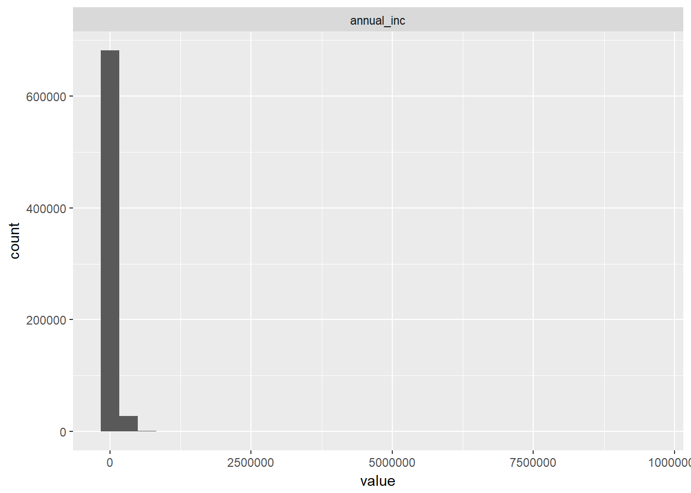
We can see that a lot of loans have corresponding annual income of zero and in general income seems low. As already known, joint income has a large number of NA values (i.e. cannot be displayed) and those few values that are present do not seem to have significant exposure. Most loan applications must have been submitted by single income borrowers, i.e. either single persons or single-income households.
train %>%
  select_(.dots = loan_amount_vars) %>%
  gather_("variable", "value", gather_cols = loan_amount_vars) %>%
  ggplot(aes(x = value)) +
  facet_wrap(~ variable, scales = "free_x", ncol = 3) +
  geom_histogram()
## `stat_bin()` using `bins = 30`. Pick better value with `binwidth`.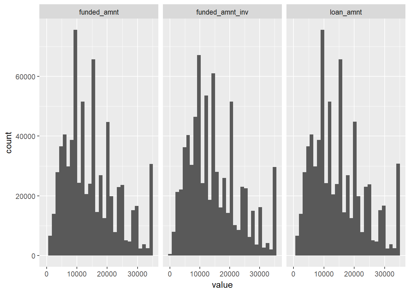
The loan amount distributions seems similar in shape suggesting not too much divergence between the loan amount applied for, the amount committed and the amount invested.
We had already identified a number of interesting categorical variables. Let’s combine our selection with the meta information gathered in an earlier stage to see the information power and uniqueness.
categorical_vars <-
  c("term", "grade", "sub_grade", "emp_title", "home_ownership",
    "verification_status", "loan_status", "purpose", "zip_code",
    "addr_state", "application_type", "policy_code")

meta_loans %>%
  select(variable, p_zeros, p_na, type, unique) %>%
  filter_(~ variable %in% categorical_vars) %>%
knitr::kable()| variable | p_zeros | p_na | type | unique |
|---|---|---|---|---|
| term | 0 | 0.0 | character | 2 |
| grade | 0 | 0.0 | character | 7 |
| sub_grade | 0 | 0.0 | character | 35 |
| emp_title | 0 | 5.8 | character | 289148 |
| home_ownership | 0 | 0.0 | character | 6 |
| verification_status | 0 | 0.0 | character | 3 |
| loan_status | 0 | 0.0 | character | 10 |
| purpose | 0 | 0.0 | character | 14 |
| zip_code | 0 | 0.0 | character | 935 |
| addr_state | 0 | 0.0 | character | 51 |
| policy_code | 0 | 0.0 | numeric | 1 |
| application_type | 0 | 0.0 | character | 2 |
This gives us some ideas on what may be useful for a broad data exploration. Variables such as emp_title have too many unique values to be suitable for a classical categorical graph. Other variables may lend themselves to pairwise or correlation graphs such as int_rate while again others may be used in time series plots such as issue_d. We may even be able to plot some appealing geographical plots with geolocation variables such as zip_code or addr_state.
9.1 Grade
For a start, let’s look at grade which seems to be a rating classification scheme that Lending Club uses to assign loans into risk buckets similar to other popular rating schemes like S&P or Moodys. For more details, see Lending Club Rate Information. For now, it suffices to know that grades take values A, B, C, D, E, F, G where A represents the highest quality loan and G the lowest.
As a first relation, we investigate the distribution of loan amount over the different grades with a standard boxplot highlighting potential outliers in red. One may also select a pre-defined theme from the ggthemes package by adding a call to ggplot such as theme_economist() or even create a theme oneself. For details on themes, see ggplot2 themes and Introduction to ggthemes.
As mentioned before we want to be group size aware so let’s write a short function to be used inside the ggplot::geom_boxplot() call in combination with ggplot::stat_summary() where we can call user-defined functions using parameter fun.data. As it is often the case with plots, we need to experiment with the position of additional text elements which we achieve by scaling the y-position with some constant multiplier around the median (as the boxplot will have the median as horizontal bar within the rectangles). The mean can be added in a similar fashion, however we don’t need to specify the y-position explicitly. The count as text and the mean as point may overlap themselves and with the median horizontal bar. This is acceptable in an exploratory setting. For publication-ready plots one would have to perform some adjustments.
# see http://stackoverflow.com/questions/15660829/how-to-add-a-number-of-observations-per-group-and-use-group-mean-in-ggplot2-boxp
give_count <-
  stat_summary(fun.data = function(x) return(c(y = median(x)*1.06,
                                               label = length(x))),
               geom = "text")

# see http://stackoverflow.com/questions/19876505/boxplot-show-the-value-of-mean
give_mean <-
  stat_summary(fun.y = mean, colour = "darkgreen", geom = "point",
               shape = 18, size = 3, show.legend = FALSE)
train %>%
ggplot(aes(grade, loan_amnt)) +
geom_boxplot(fill = "white", colour = "darkblue",
outlier.colour = "red", outlier.shape = 1) +
give_count +
give_mean +
scale_y_continuous(labels = comma) +
facet_wrap(~ default) +
labs(title="Loan Amount by Grade", x = "Grade", y = "Loan Amount \n")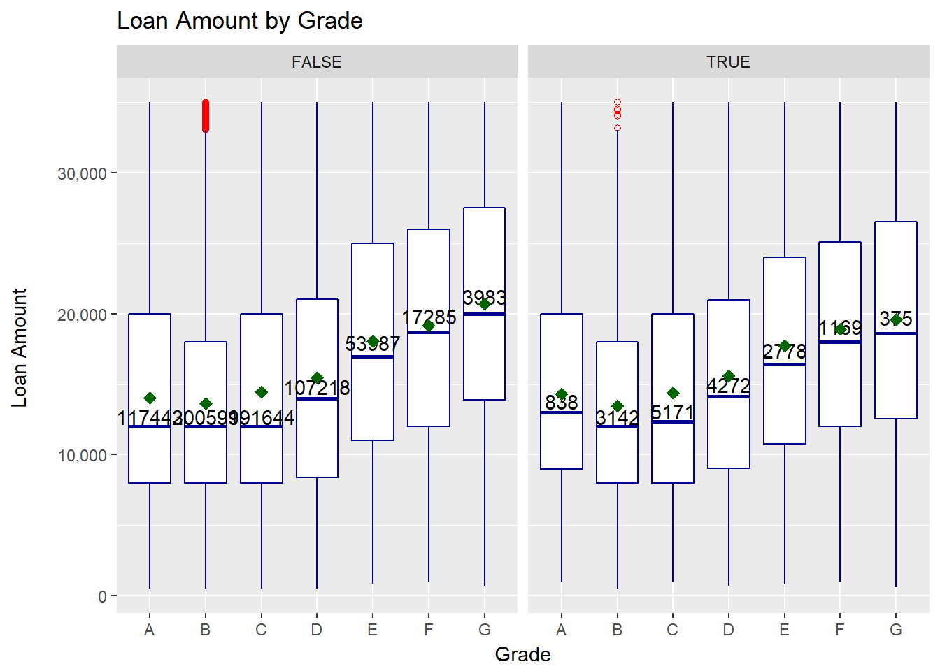
We can derive a few points from the plot:
- there is not a lot of difference between default and non-default
- lower quality loans tend to have a higher loan amount
- there are virtually no outliers except for grade B
- the loan amount spread (IQR) seems to be slightly higher for lower quality loans
According to Lending Club’s rate information, we would expect a strong increasing relationship between grade and interest rate so we can test this. We also consider the term of the loan as one might expect that longer term loans could have a higher interest rate.
train %>%
  ggplot(aes(grade, int_rate)) +
  geom_boxplot(fill = "white", colour = "darkblue",
               outlier.colour = "red", outlier.shape = 1) +
  give_count +
  give_mean +
  scale_y_continuous(labels = comma) +
  labs(title="Interest Rate by Grade", x = "Grade", y = "Interest Rate \n") +
  facet_wrap(~ term)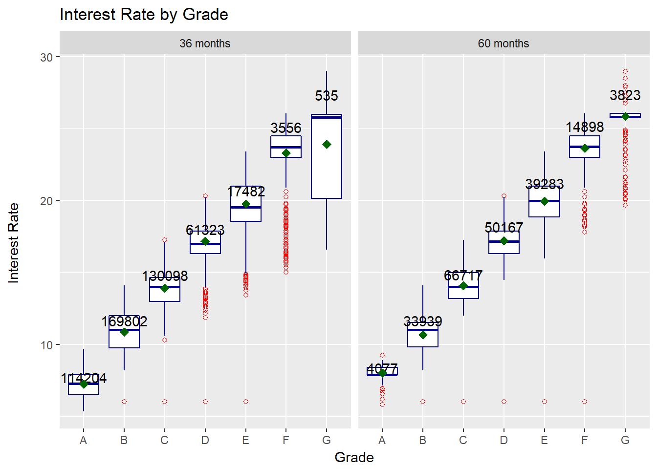
We can derive a few points from the plot:
- interest rate increases with grade worsening
- a few loans seem to have an equally low interest rate independent of grade
- the spread of rates seems to increase with grade worsening
- there tend to be more outliers on the lower end of the rate
- The 3-year term has a much higher number of high-rated borrowers while the 5-year term has a larger number in the low-rating grades
9.2 Home Ownership
We can do the same for home ownership.
train %>%
  ggplot(aes(home_ownership, int_rate)) +
  geom_boxplot(fill = "white", colour = "darkblue",
               outlier.colour = "red", outlier.shape = 1) +
  give_count +
  give_mean +
  scale_y_continuous(labels = comma) +
  facet_wrap(~ default) +
  labs(title="Interest Rate by Home Ownership", x = "Home Ownership", y = "Interest Rate \n")
We can derive a few points from the plot:
- there seems no immediate conclusion with respect to the impact of home ownership, e.g. we can see that median/mean interest rate is higher for people who own a house than for those who still pay a mortgage.
- interest rates are highest for values “any” and “none” which could be loans of limited data quality but there are very few data points.
- interest rate is higher for default loans, which is probably driven by other factors (e.g. grade)
9.3 Loan Amount and Income
Another interesting plot may be the relationship between loan amount and funded / invested amount. As all variables are continous, we can do that with a simple scatterplot but we will need to reshape the data to have both loan values plotted against loan amount.
In fact the reshaping here may be slightly odd as we like to display the same variable on the x-axis but different values on the y-axis facetted by their variable names. To achieve that, we gather the data three times with the same x variable but changing y variables.
funded_amnt <-
  train %>%
  transmute(loan_amnt = loan_amnt, value = funded_amnt,
              variable = "funded_amnt")

funded_amnt_inv <-
  train %>%
  transmute(loan_amnt = loan_amnt, value = funded_amnt_inv,
              variable = "funded_amnt_inv")

plot_data <- rbind(funded_amnt, funded_amnt_inv)
# remove unnecessary data using regex
ls()
## [1] "categorical_vars" "chr_to_date_vars" "chr_to_num_vars"
## [4] "convert_date" "default_vars" "defaulted"
## [7] "excel_file" "funded_amnt" "funded_amnt_inv"
## [10] "give_count" "give_mean" "i"
## [13] "income_vars" "libraries_missing" "libraries_used"
## [16] "loan_amount_vars" "loans" "meta_browse_notes"
## [19] "meta_loan_stats" "meta_loans" "meta_reject_stats"
## [22] "na_to_zero_vars" "num_vars" "path"
## [25] "plot_data" "test" "train"
## [28] "train_index" "vars_to_remove"rm(list = ls()[grep("^funded", ls())])Now let’s plot the data.
plot_data %>%
  ggplot(aes(x = loan_amnt, y = value)) +
  facet_wrap(~ variable, scales = "free_x", ncol = 3) +
  geom_point()
We can derive a few points from the plot:
- there are instances when funded amount is smaller loan amount
- there seems to be a number of loans where investment is smaller funded amount i.e. not the full loan is invested in
Let’s do the same but only for annual income versus loan amount.
train %>%
  ggplot(aes(x = annual_inc, y = loan_amnt)) +
  geom_point()
## Warning: Removed 4 rows containing missing values (geom_point).
We can derive a few points from the plot:
- there is no immediatly discernible relationship
- there are quite a few income outliers with questionable values (e.g. why would a person with annual income 9500000 request a loan amount of 24000)
9.4 Time Series
Now let’s take a look at interest rates over time but split the time series by grade to see if there are differences in interest rate development depending on the borrower grade. Again we make use of a dplyr pipe, first selecting the variables of interest, then grouping by attributes and finally summarising the metric interest rate by taking the mean for each goup. We use facet_wrap to split by attribute grade. As we are using the mean for building an aggregate representation, we should be weary of outliers and group size which we had already looked at earlier (ignoring time dimension).
train %>%
  select(int_rate, grade) %>%
  group_by(grade) %>%
  summarise(int_rate_mean = mean(int_rate, na.rm = TRUE),
            int_rate_median = median(int_rate, na.rm = TRUE),
            n = n()) %>%
knitr::kable()| grade | int_rate_mean | int_rate_median | n |
|---|---|---|---|
| A | 7.244639 | 7.26 | 118281 |
| B | 10.830884 | 10.99 | 203741 |
| C | 13.979427 | 13.98 | 196815 |
| D | 17.178566 | 16.99 | 111490 |
| E | 19.899484 | 19.99 | 56765 |
| F | 23.572306 | 23.76 | 18454 |
| G | 25.624502 | 25.83 | 4358 |
Group size are relatively large except for grade G which may have only a few hundred loans per group when grouping by grade and date. Mean and median seem fairly close at this non-granular level. Let’s plot the data.
train %>%
  select(int_rate, grade, issue_d) %>%
  group_by(grade, issue_d) %>%
  summarise(int_rate_mean = mean(int_rate, na.rm = TRUE)) %>%
  ggplot(aes(issue_d, int_rate_mean)) +
  geom_line(color= "darkblue", size = 1) +
  facet_wrap(~ grade)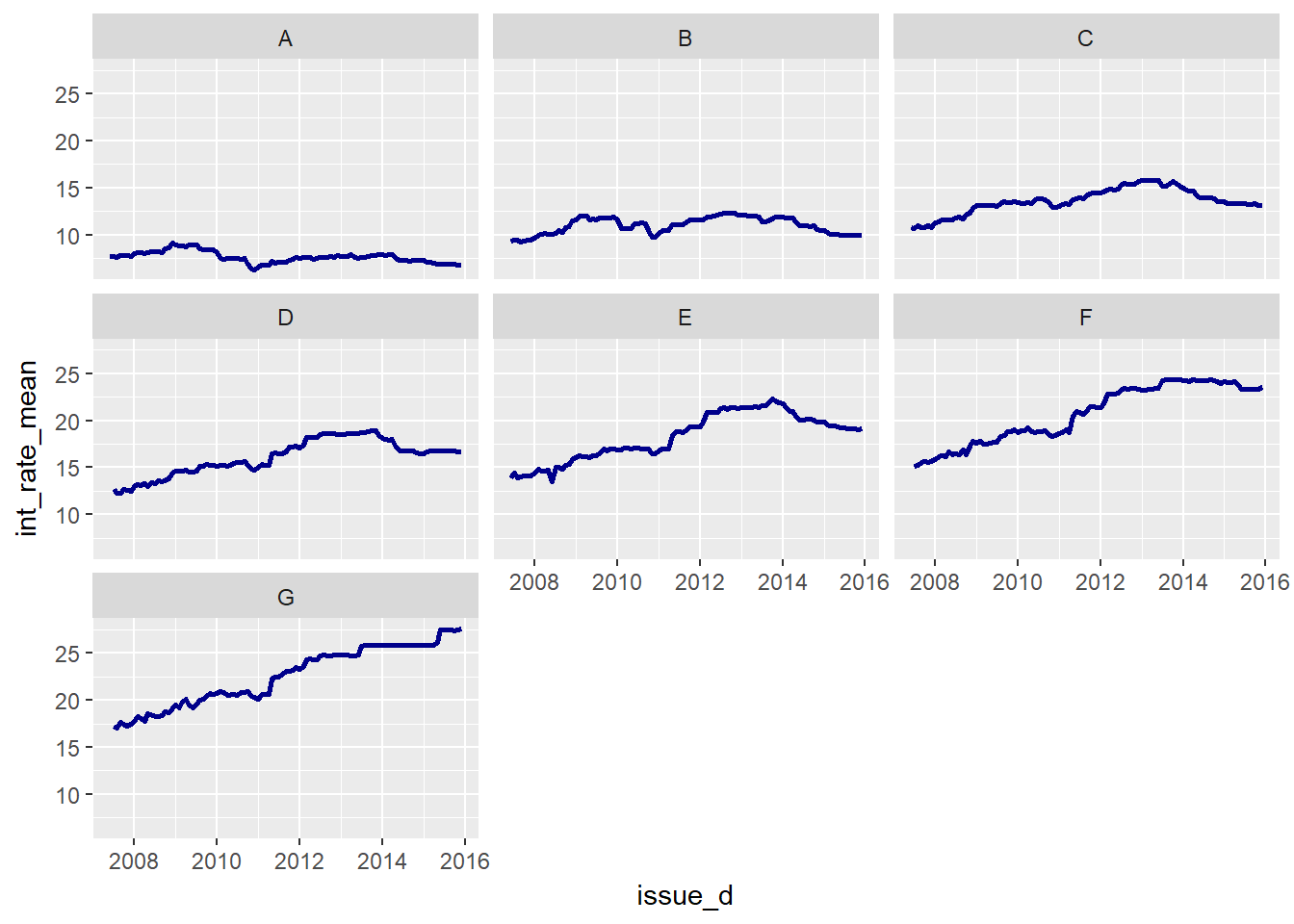
We can derive a few points from the plot:
- the mean interest rate is falling or relatively constant for high-rated clients
- the mean interest rate is increasing significantly for low-rated clients
Let’s also look at loan amounts over time in the same manner.
train %>%
  select(loan_amnt, grade, issue_d) %>%
  group_by(grade, issue_d) %>%
  summarise(loan_amnt_mean = mean(loan_amnt, na.rm = TRUE)) %>%
  ggplot(aes(issue_d, loan_amnt_mean)) +
  geom_line(color= "darkblue", size = 1) +
  facet_wrap(~ grade)
We can derive a few points from the plot:
- the mean loan amount is increasing for all grades
- while high-rated clients have some mean loan amount volatility, it is much higher for low-rated clients
9.5 Geolocation Plots
Let’s remind ourselves of the geolocation variables in the data and their information power.
- zip_code (geo-info)
- addr_state (geo-info)
geo_vars <- c("zip_code", "addr_state")

meta_loans %>%
  select(variable, p_zeros, p_na, type, unique) %>%
  filter_(~ variable %in% geo_vars) %>%
knitr::kable()| variable | p_zeros | p_na | type | unique |
|---|---|---|---|---|
| zip_code | 0 | 0 | character | 935 |
| addr_state | 0 | 0 | character | 51 |
loans %>%
  select_(.dots = geo_vars) %>%
  str()
## Classes 'tbl_df', 'tbl' and 'data.frame': 887379 obs. of 2 variables:
## $ zip_code : chr "860xx" "309xx" "606xx" "917xx" ...
## $ addr_state: chr "AZ" "GA" "IL" "CA" ...We see that zip_code seems to be the truncated US postal code with only first three digits having a value. The addr_state seems to be the state names in a two-letter abbreviation.
We can use the choroplethr package to work with maps (alternatives may be maps among other packages). While choroplethr provides functions to work with the data, its sister package choroplethrMaps contains corresponding maps that can be used by choroplethr. One issue with choroplethr is that it attaches the package plyr which means many functions from dplyr are masked as it is the successor to plyr. Thus we do not load the package choroplethr despite using its functions frequently. However, we need to load choroplethrMaps as it has some data that is not exported from its namespace so syntax like choroplethrMaps::state.map where state.map is the rdata file does not work. An alternative might be to load the file directly by going to the underlying directory, e.g. R-3.x.x\library\choroplethrMaps\data but this is cumbersome. As discussed before, when attaching a library, we just need to make sure that important functions of other packages are not masked. In this case it’s fine.
For details on those libraries, see CRAN choroplethr and CRAN choroplethrMaps.
First we aggregate the default rate by state.
default_rate_state <-
  train %>%
  select(default, addr_state) %>%
  group_by(addr_state) %>%
  summarise(default_rate = sum(default, na.rm = TRUE) / n())

knitr::kable(default_rate_state)| addr_state | default_rate |
|---|---|
| AK | 0.0289280 |
| AL | 0.0300944 |
| AR | 0.0243994 |
| AZ | 0.0260203 |
| CA | 0.0247008 |
| CO | 0.0233654 |
| CT | 0.0222655 |
| DC | 0.0131646 |
| DE | 0.0291604 |
| FL | 0.0267678 |
| GA | 0.0238065 |
| HI | 0.0303441 |
| IA | 0.2000000 |
| ID | 0.0000000 |
| IL | 0.0201743 |
| IN | 0.0242243 |
| KS | 0.0162975 |
| KY | 0.0204172 |
| LA | 0.0268172 |
| MA | 0.0246096 |
| MD | 0.0279492 |
| ME | 0.0023474 |
| MI | 0.0249429 |
| MN | 0.0239122 |
| MO | 0.0222711 |
| MS | 0.0301540 |
| MT | 0.0289296 |
| NC | 0.0263557 |
| ND | 0.0075377 |
| NE | 0.0156087 |
| NH | 0.0206490 |
| NJ | 0.0249566 |
| NM | 0.0264766 |
| NV | 0.0303213 |
| NY | 0.0294889 |
| OH | 0.0225960 |
| OK | 0.0283897 |
| OR | 0.0209814 |
| PA | 0.0256838 |
| RI | 0.0245849 |
| SC | 0.0218611 |
| SD | 0.0301164 |
| TN | 0.0267720 |
| TX | 0.0240810 |
| UT | 0.0250696 |
| VA | 0.0279697 |
| VT | 0.0172771 |
| WA | 0.0216223 |
| WI | 0.0213508 |
| WV | 0.0225434 |
| WY | 0.0179455 |
The data is already in a good format but when using choroplethr we need to adhere to some conventions to make it work out of the box. The first thing would be to bring the state names into a standard format. In fact, we can investigate the format by looking e.g. into the choroplethrMaps::state.map dataset which we later use to map our data. We first load the library and then the data via the function utils::data(). From the documentation, we also learn that state.map is a “data.frame which contains a map of all 50 US States plus the District of Columbia.” It is based on a shapefile which is often used in geospatial visualizations and “taken from the US Census 2010 Cartographic Boundary shapefiles page”. We are interested in the region variable which seems to hold the state names.
library(choroplethrMaps)
utils::data(state.map)
str(state.map)
## 'data.frame': 50763 obs. of 12 variables:
## $ long : num -113 -113 -112 -112 -111 ...
## $ lat : num 37 37 37 37 37 ...
## $ order : int 1 2 3 4 5 6 7 8 9 10 ...
## $ hole : logi FALSE FALSE FALSE FALSE FALSE FALSE ...
## $ piece : Factor w/ 66 levels "1","2","3","4",..: 1 1 1 1 1 1 1 1 1 1 ...
## $ group : Factor w/ 226 levels "0.1","1.1","10.1",..: 1 1 1 1 1 1 1 1 1 1 ...
## $ id : chr "0" "0" "0" "0" ...
## $ GEO_ID : Factor w/ 51 levels "0400000US01",..: 3 3 3 3 3 3 3 3 3 3 ...
## $ STATE : Factor w/ 51 levels "01","02","04",..: 3 3 3 3 3 3 3 3 3 3 ...
## $ region : chr "arizona" "arizona" "arizona" "arizona" ...
## $ LSAD : Factor w/ 0 levels: NA NA NA NA NA NA NA NA NA NA ...
## $ CENSUSAREA: num 113594 113594 113594 113594 113594 ...unique(state.map$region)## [1] "arizona" "arkansas" "louisiana"
## [4] "minnesota" "mississippi" "montana"
## [7] "new mexico" "north dakota" "oklahoma"
## [10] "pennsylvania" "tennessee" "virginia"
## [13] "california" "delaware" "west virginia"
## [16] "wisconsin" "wyoming" "alabama"
## [19] "alaska" "florida" "idaho"
## [22] "kansas" "maryland" "colorado"
## [25] "new jersey" "north carolina" "south carolina"
## [28] "washington" "vermont" "utah"
## [31] "iowa" "kentucky" "maine"
## [34] "massachusetts" "connecticut" "michigan"
## [37] "missouri" "nebraska" "nevada"
## [40] "new hampshire" "new york" "ohio"
## [43] "oregon" "rhode island" "south dakota"
## [46] "district of columbia" "texas" "georgia"
## [49] "hawaii" "illinois" "indiana"So it seems we need small case long form state names which implies we need a mapping from the short names in our data. Some internet research may give us the site American National Standards Institute (ANSI) Codes for States where we find a mapping under section FIPS Codes for the States and the District of Columbia. We could try using some parsing tool to extract the table from the web page but for now we take a short cut and simply copy paste the data into a tab-delimited txt file and read the file with readr::read_tsv(). We then cross-check if all abbreviations used in our loans data are present in the newly created mapping table.
states <- readr::read_tsv("./data//us_states.txt")## Parsed with column specification:
## cols(
## Name = col_character(),
## `FIPS State Numeric Code` = col_integer(),
## `Official USPS Code` = col_character()
## )str(states)## Classes 'tbl_df', 'tbl' and 'data.frame': 51 obs. of 3 variables:
## $ Name : chr "Alabama" "Alaska" "Arizona" "Arkansas" ...
## $ FIPS State Numeric Code: int 1 2 4 5 6 8 9 10 11 12 ...
## $ Official USPS Code : chr "AL" "AK" "AZ" "AR" ...
## - attr(*, "spec")=List of 2
## ..$ cols :List of 3
## .. ..$ Name : list()
## .. .. ..- attr(*, "class")= chr "collector_character" "collector"
## .. ..$ FIPS State Numeric Code: list()
## .. .. ..- attr(*, "class")= chr "collector_integer" "collector"
## .. ..$ Official USPS Code : list()
## .. .. ..- attr(*, "class")= chr "collector_character" "collector"
## ..$ default: list()
## .. ..- attr(*, "class")= chr "collector_guess" "collector"
## ..- attr(*, "class")= chr "col_spec"# give some better variable names (spaces never helpful)
names(states) <- c("name", "fips_code", "usps_code")
# see if all states are covered
dplyr::setdiff(default_rate_state$addr_state, states$usps_code)## character(0)Comparing the unique abbreviations in the loans data with the usps codes reveals that we are all covered so let’s bring the data together using dplyr::left_join(). For details on dplyr join syntax, see Two-table verbs. To go with the choroplethr conventions, we also need to
- have state names in lower case
- rename the mapping variable to
regionand the numeric metric tovalue. - only select above two variables in the function call
Note that we are re-assigning the data to itself to avoid creating a new table.
default_rate_state <-
  default_rate_state %>%
  left_join(states[, c("usps_code", "name")],
            by = c("addr_state" = "usps_code")) %>%
  rename(region = name, value = default_rate) %>%
  mutate(region = tolower(region)) %>%
  select(region, value)
Finally, we can plot the data using the default colors from choroplethr. As we are having data on state level, we use function choroplethr::state_choropleth().
choroplethr::state_choropleth(df = default_rate_state,
                              title = "Default rate by State")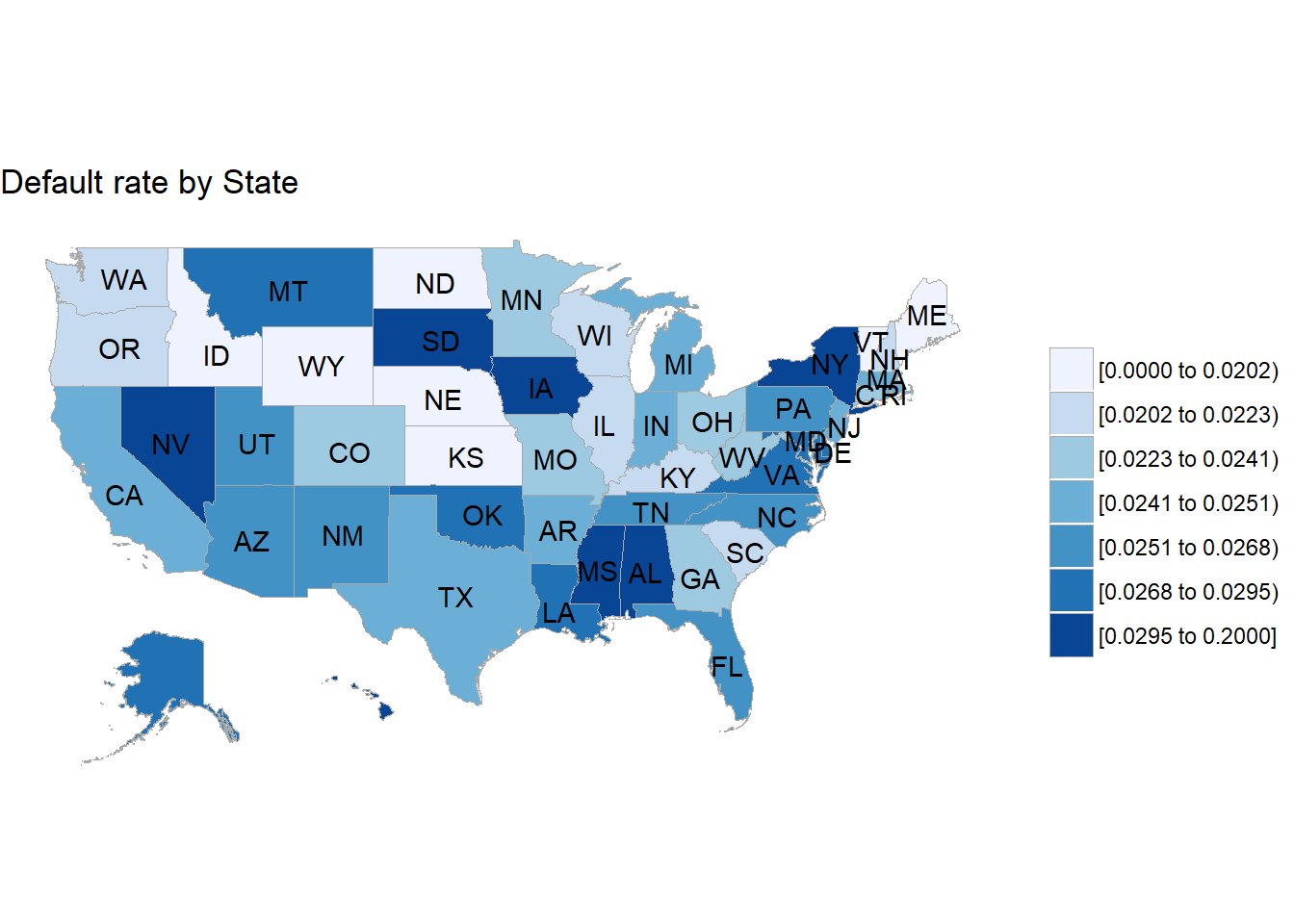
We can derive a few points from the plot:
- default rate varies across states
- we may want to adjust the default binning
- we are only looking at default rate but not defaulted exposure (there may be states with many defaults but the defaulted amount is small)
We could do the same exercise but on a more granular level as we have zip codes available. They are truncated so we would have to find a way to work with them. They also have a high number of unique values so the map legend may be cramped if we were looking at all of US.
10 Correlation
Many models rely on the notion of correlation between independent and dependent variables so a natural exploratoy visualization would be a correlation plot or correlogram. One library offering this is corrplot with its main function corrplot::corrplot(). The function takes as input the correlation matrix that can be produced with stats::cor(). This of course is only defined for numeric, non-missing variables. In order to have a reasonable information density in the correlation matrix, we will kick out some variables with a missing value share of larger 50%.
For a discussion on missing value treatment, see e.g. Data Analysis Using Regression and Multilevel/Hierarchical Models - Chapter 25: Missing-data imputation
Let’s again build a numeric variable vector after all previous operations and look at correlations.
num_vars <-
  train %>%
  sapply(is.numeric) %>%
  which() %>%
  names()

meta_train <- funModeling::df_status(train, print_results = FALSE)

meta_train %>%
  select(variable, p_zeros, p_na, unique) %>%
  filter_(~ variable %in% num_vars) %>%
knitr::kable()| variable | p_zeros | p_na | unique |
|---|---|---|---|
| loan_amnt | 0.00 | 0.00 | 1369 |
| funded_amnt | 0.00 | 0.00 | 1369 |
| funded_amnt_inv | 0.03 | 0.00 | 8203 |
| int_rate | 0.00 | 0.00 | 540 |
| installment | 0.00 | 0.00 | 64438 |
| annual_inc | 0.00 | 0.00 | 41978 |
| dti | 0.05 | 0.00 | 4072 |
| delinq_2yrs | 80.80 | 0.00 | 26 |
| inq_last_6mths | 56.10 | 0.00 | 27 |
| mths_since_last_delinq | 51.43 | 0.00 | 152 |
| mths_since_last_record | 84.70 | 0.00 | 123 |
| open_acc | 0.00 | 0.00 | 74 |
| pub_rec | 84.70 | 0.00 | 31 |
| revol_bal | 0.38 | 0.00 | 68979 |
| revol_util | 0.40 | 0.05 | 1312 |
| total_acc | 0.00 | 0.00 | 131 |
| out_prncp | 28.85 | 0.00 | 209810 |
| out_prncp_inv | 28.85 | 0.00 | 224620 |
| total_pymnt | 2.01 | 0.00 | 423038 |
| total_pymnt_inv | 2.04 | 0.00 | 424921 |
| total_rec_prncp | 2.05 | 0.00 | 222003 |
| total_rec_int | 2.06 | 0.00 | 287778 |
| total_rec_late_fee | 98.59 | 0.00 | 5169 |
| recoveries | 97.22 | 0.00 | 18681 |
| collection_recovery_fee | 97.35 | 0.00 | 16796 |
| last_pymnt_amnt | 2.00 | 0.00 | 197434 |
| collections_12_mths_ex_med | 98.65 | 0.02 | 12 |
| mths_since_last_major_derog | 75.06 | 0.00 | 167 |
| acc_now_delinq | 99.53 | 0.00 | 8 |
| tot_coll_amt | 78.94 | 7.92 | 9319 |
| tot_cur_bal | 0.01 | 7.92 | 293158 |
Finally, we can produce a correlation plot. Dealing with missing values, using option use = "pairwise.complete.obs" in function stats::cor() is considered bad practice as it uses pair matching and correlations may not be comparable, see e.g. Pairwise-complete correlation considered dangerous. Alternatively, we can use option use = complete.obs which only considers complete observations but may discard a lot of data. However, as we have looked into the meta information, after our wrangling the proportion of missing values for the numeric variables has dropped a lot so we should be fine.
Once we have the correlation matrix, we can use the function corrplot::corrplot() from the corrplot library. It offers a number of different visualization options. For details, see An Introduction to corrplot Package.
library(corrplot)
corrplot::corrplot(cor(train[, num_vars], use = "complete.obs"),
                   method = "pie", type = "upper")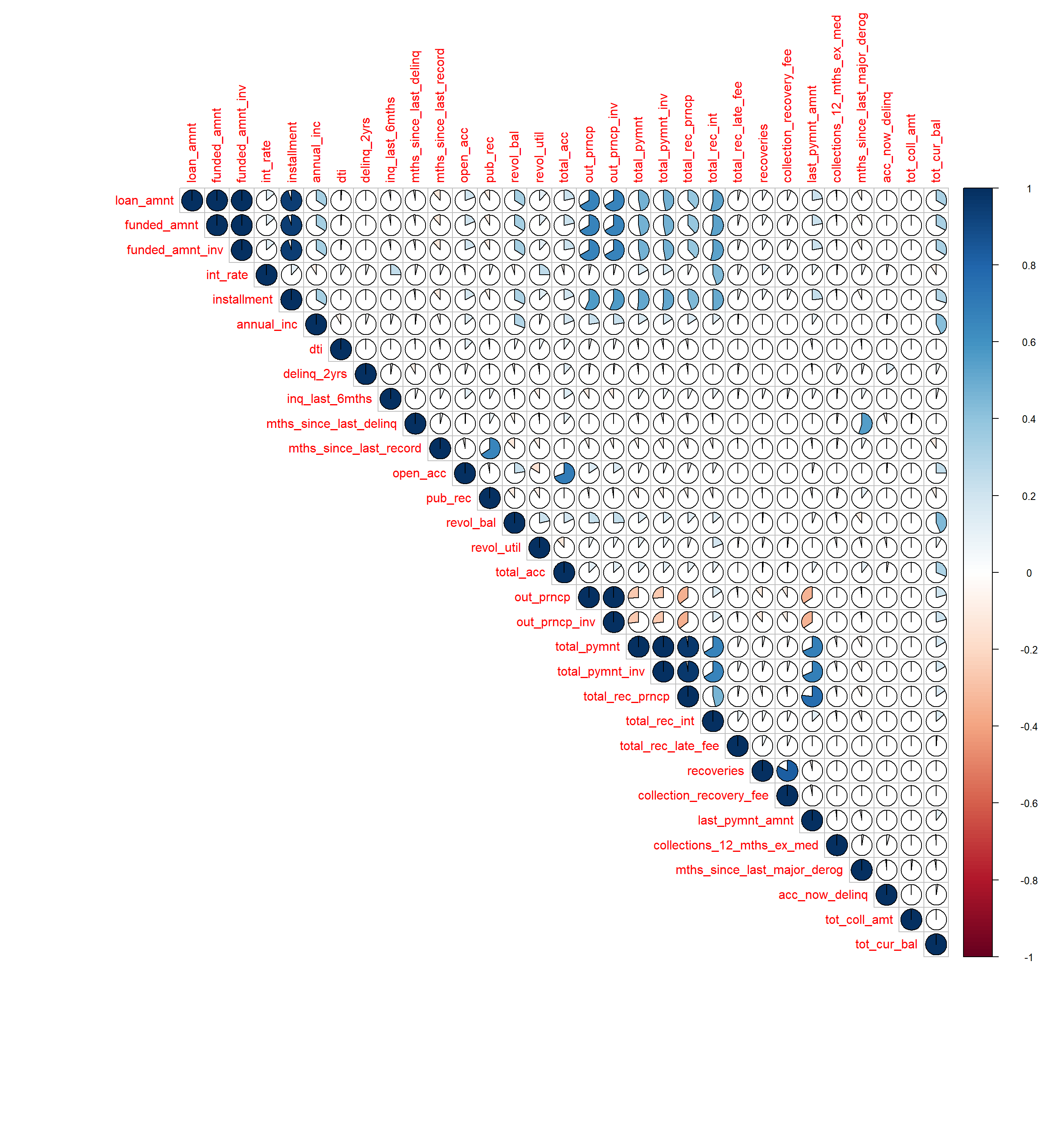
We can derive a few things from the plot
- overall correlation between variables seems low but there are a few highly correlated ones
- some highly correlated variables may indicate very similar information, e.g.
mths_since_last_delinqandmths_since_last_major_derog - some variables are perfectly correlated and thus should be removed
Rather than a visual inspection, an (automatic) inspection of correlations and removal of highly correlated features can be done via function caret::findCorrelation() with a defined cutoff parameter. If two variables have a high correlation, the function looks at the mean absolute correlation of each variable and removes the variable with the largest mean absolute correlation. Using exact = TRUE will cause the function to re-evaluate the average correlations at each step while exact = FALSE uses all the correlations regardless of whether they have been eliminated or not. The exact calculations will remove a smaller number of predictors but can be much slower when the problem dimensions are “big”.
caret::findCorrelation(cor(train[, num_vars], use = "complete.obs"),
                       names = TRUE, cutoff = .5)
## [1] "loan_amnt" "funded_amnt"
## [3] "funded_amnt_inv" "installment"
## [5] "total_pymnt_inv" "total_pymnt"
## [7] "total_rec_prncp" "out_prncp"
## [9] "total_acc" "mths_since_last_record"
## [11] "mths_since_last_major_derog" "recoveries"Given above, we remove a few variables
vars_to_remove <-
  c("loan_amnt", "funded_amnt", "funded_amnt_inv", "installment",
    "total_pymnt_inv", "total_rec_prncp", "mths_since_last_delinq",
    "out_prncp", "total_pymnt", "total_rec_int", "total_acc",
    "mths_since_last_record", "recoveries")

train <- train %>% select(-one_of(vars_to_remove))
11 Summary plots
An alternative to producing individual exploratory plots is using summary plots that come with sensible default settings and display the data according to its data type (numeric or categorical). The advantages are that a lot of information can be put into one graph and potential relationships may be spotted more easily. The disadvantages are potential performance issues when plotting many variables of a large dataset and readability issues in case of many dimensions for categorical variables. These disadvantages can be somewhat remediated by looking at summary plots after a lot of variables have already been discarded due to other findings (as we have done here). To show the general idea, we use the GGally library which builds on top of ggplot2 and provides some nice visualization functions. We choose a subset of variables for illustration of the GGally::ggpairs() function. Even with this subset the production of the graph may take some time depending on your hardware. For a theoretical background, see The Generalized Pairs Plot. For the many customization options, see GGally. As always when visualizing a lot of information, there is a trade-off between information density and visualization efficiency. The more variables are selected for the plot, the more difficult it becomes to efficiently visualize it. This needs some playing around or a really big screen.
Note
Simply leaving the variable
defaultas boolean would produce an error inggpairs(or rather inggplot2which it calls):Error: StatBin requires a continuous x variable the x variable is discrete. Perhaps you want stat="count"?. Besides, we like it to be treated as categorical so we convert it to character for this function call.
library(GGally)
plot_ggpairs <-
  train %>%
  select(annual_inc, term, grade, default) %>%
  mutate(default = as.character(default)) %>%
  ggpairs()

plot_ggpairs
The resulting graph has a lot of information in it and we won’t go into further detail here but the most important points to read the graph properly. In the columns:
- for single continuous numeric variable plots density estimate
- for continuous numeric variable against another continuous numeric variable plots scatterplot
- for continuous numeric variable against another categorical variable plots histogram
- for single categorical variable plots histogram
In the rows:
- for continuous numeric variable against another continuous numeric variable plots correlation
- for continuous numeric variable against another categorical variable plots boxplot by dimension of categorical variable
- for categorical variable against another categorical variable plots historgram by dimension of y-axis categorical variable
- for categorical variable against another continuous variable plots scatterplot by dimension of categorical variable
Another interesting plot would be to visualize the density (estimates) of the numeric variables color-coded by the classes of the target variable (here: default/non-default) to inspect whether there are visual clues about differences in the distributions. We can achieve this by using ggplot but need to bring the data into a long format rather than its current wide format (see Data Science with R - Chapter Data Tidying for details on reshaping). We use tidyr::gather() to bring the numeric variables into a long format and then add the target variable again. Note that there are different lengths of the reshaped data and the original target variable vector. As dplyr::mutate() will not properly take care of the recycling rules, we have to recycle (repeat) the variable default manually to have the same length as the reshaped train data. See An Introduction to R - Chapter 2.2: Vector arithmetic how recycling works in general.
Vectors occurring in the same expression need not all be of the same length. If they are not, the value of the expression is a vector with the same length as the longest vector which occurs in the expression. Shorter vectors in the expression are recycled as often as need be (perhaps fractionally) until they match the length of the longest vector. In particular a constant is simply repeated.
Note that we make use of a few plot parameters to make the visualization easier to follow. We like default to be a factor so the densities are independent of class distribution. First, we switch the levels of variable default to have TRUE on top (as the highest objective is to get the true positive right). We use the fill and color parameters to encode with the target variable. This allows a visual distinction of overlaying densities. In addition, we set the alpha value to have the area under the curve transparently filled. For color selection we make use of brewer scales which offer a well selected pallette of colors. Finally, we split the plots by variable with facet_wrap allowing the scales of each indifidual plot to be free and defining the number of columns via ncol.
num_vars <- train %>% sapply(is.numeric) %>% which() %>% names()

train %>%
  select_(.dots = num_vars) %>%
  gather(measure, value) %>%
  mutate(default = factor(rep(x = train$default,
                              length.out = length(num_vars) * dim(train)[1]),
                          levels = c("TRUE", "FALSE"))) %>%
  ggplot(data = ., aes(x = value, fill = default,
                       color = default, order = -default)) +
  geom_density(alpha = 0.3, size = 0.5) +
  scale_fill_brewer(palette = "Set1") +
  scale_color_brewer(palette = "Set1") +
  facet_wrap( ~ measure, scales = "free", ncol = 3)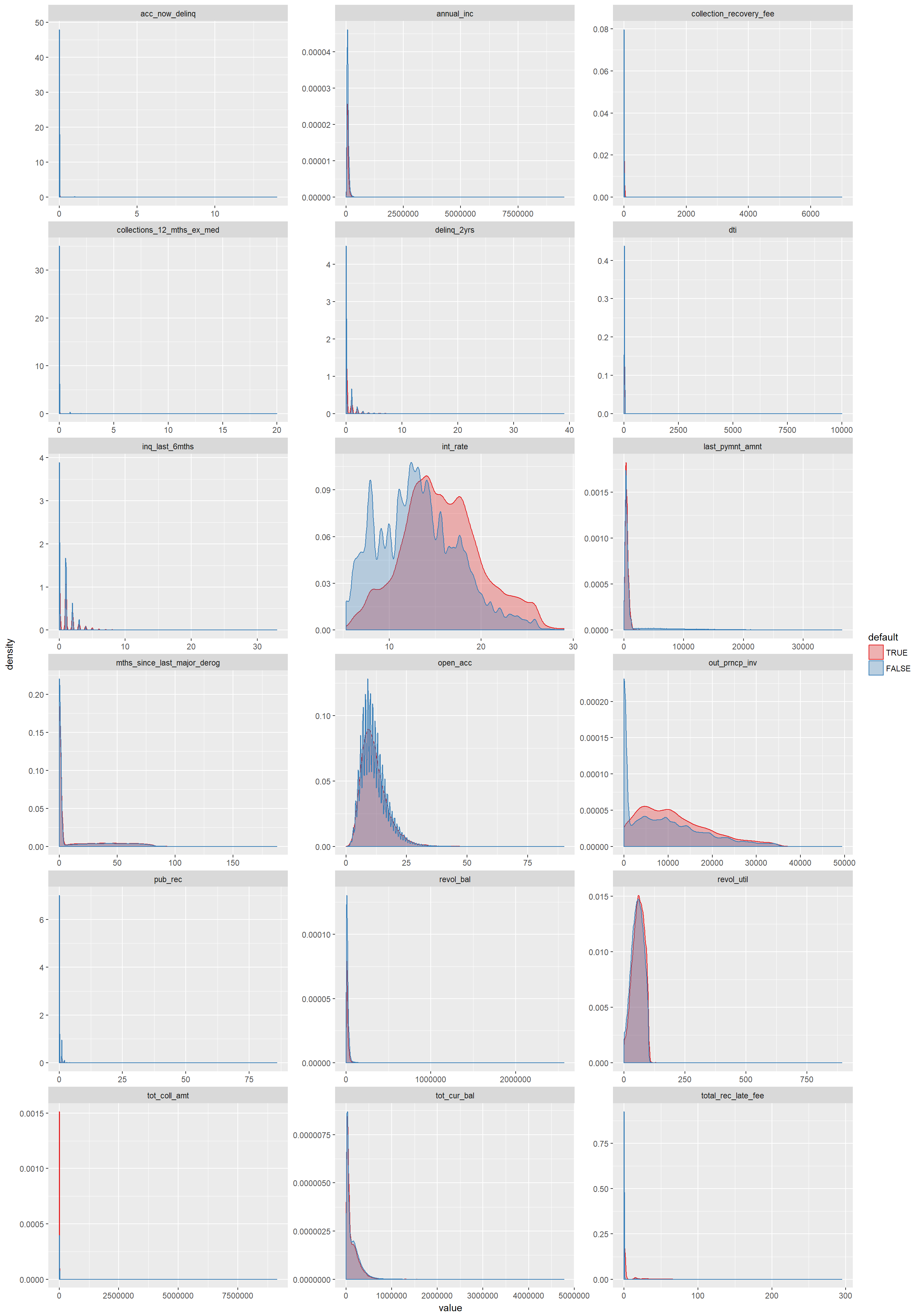
We can derive a few things from the plot:
- most of the densities are right-skewed with probably a few outliers extending the x-axis which makes discerning patterns in the area with highest mass difficult
- even with above mentioned visualization impediment it seems that there is not a lot of difference between default and non-default loans for most variables
- some densities seem wobbly for the majority class (e.g.
open_acc) which is caused by the fact that the smoothing algorithm has many more data points to smooth in between but the density follows the same general shape
Given above observations, we can try to improve the plot by removing (adjusting) outliers. There are many different methods that can be used, see e.g.
- A Survey of Outlier Detection Methodologies
- On Evaluation of Outlier Rankings and Outlier Scores
- Outliers: An Evaluation of Methodologies
- A protocol for data exploration to avoid common statistical problems
- Outlier detection and treatment with R
- Data Mining and Knowledge Discovery Handbook - Chapter 1: Outlier Detection
Most of these methods focus on removing outliers for modeling which requires a lot of care and understanding how model characteristics change when removing / replacing outliers. In our case, we can be more pragmatic as we are only interested in improving our understanding of the mass of the distribution in a graphical way to see if there are easily discernible pattern differences between the two outcomes of our target variable. For this, we like to replace outliers with some sensible value derived from the distribution of the particular variable. One could use the interquartile range as it is used in boxplots. We will use winsorization, i.e. replacing outliers with a specified percentile, e.g. 95%. As this is a fairly simple task, we write our own function to do that. Alternatively, one may use e.g. function psych::winsor() which trims outliers from both ends of the distribution. Since we have already seen, that there is no negative value present, we only cut from the right side of the distribution. We call the function winsor_outlier and allow settings for the percentile and removing NA values. The design is inspired by an SO question How to replace outliers with the 5th and 95th percentile values in R.
winsor_outlier <- function(x, cutoff = .95, na.rm = FALSE){
    quantiles <- quantile(x, cutoff, na.rm = na.rm)
    x[x > quantiles] <- quantiles
    x
    }

train %>%
  select_(.dots = num_vars) %>%
  mutate_all(.funs = winsor_outlier, cutoff = .95, na.rm = TRUE) %>%
  gather(measure, value) %>%
  mutate(default = factor(rep(x = train$default,
                              length.out = length(num_vars)*dim(train)[1]),
                          levels = c("TRUE", "FALSE"))) %>%
  ggplot(data = ., aes(x = value, fill = default,
                       color = default, order = -default)) +
  geom_density(alpha = 0.3, size = 0.5) +
  scale_fill_brewer(palette = "Set1") +
  scale_color_brewer(palette = "Set1") +
  facet_wrap( ~ measure, scales = "free", ncol = 3)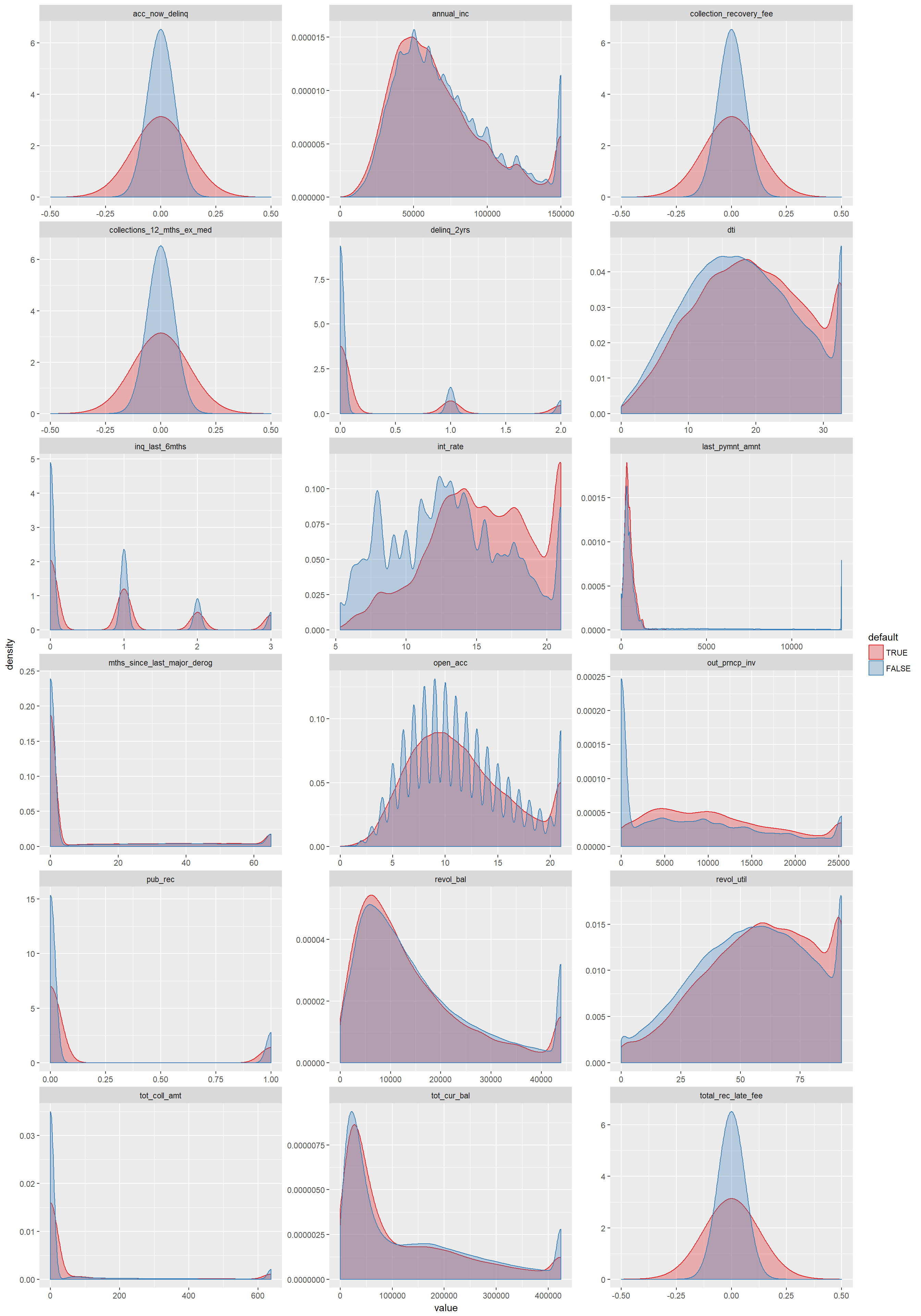
We can derive a few things from the plot:
- most densities don’t show a discernible difference between default and non-default
- ignore the densities centered around zero as they stem from too few observations
- some densities show a bump on the right stemming from the outlier replacement and thus indicating that there is actually data in the tail
Interestingly, variable out_prncp_inv shows a significant bump around zero for default == FALSE which can be confirmed via a count. However, the description tells us that this variable represents Remaining outstanding principal for portion of total amount funded by investors so it’s unclear how useful it is (especially when knowing that this variable will only be available after a loan has been granted).
train %>%
  select(default, out_prncp_inv) %>%
  filter(out_prncp_inv == 0) %>%
  group_by(default) %>%
  summarize(n = n())
## # A tibble: 2 x 2
## default n
## <lgl> <int>
## 1 FALSE 204207
## 2 TRUE 613Overall, it seems from visual inspection that the numeric variables do not contain a lot of information gain regarding the classification of the target variable. One obvious exception is the interest rate which is a function of the expected risk of the borrower probably mostly driven by the rating. Here we see that defaulted clients tend to have higher interest rates and also seem to have more outliers in the tail.
A side note on plotting
If your screen is too small, you can export any plot to e.g. svg or pdf using graphics devices of the cairo API in package grDevices (usually part of base R distro) and scale the plot size to something bigger (especially helpful if it’s a long plot). Here we show an example for the previously created ggpairs plot stored as pdf.
cairo_pdf(filename = paste0(path, "/plot_ggpairs.pdf"),
    width=15,
    height=20,
    pointsize=10)
plot_ggpairs
dev.off()
12 Modeling
12.1 Model options
There are a couple of different model options available for a supervised binary classification problem such as determining whether a loan will default or not. In general, we may distinguish the following model approaches (among others):
- logistic regression
- linear discriminant analysis
- k-nearest neighbors (kNN)
- trees
- random forests
- boosting
- support vector machines (SVM)
In addition, there are multiple ways to assess model performance such as model parameters, cross-validation, bootstrap and multiple feature selection methods such as ridge regression, the lasso, principal component anaylsis, etc.
We will look at some of those models and methods and see how they compare. For a more detailed treatment and further background, an accessible text is “An Introduction to Statistical Learning” or for a more advanced treatment “The Elements of Statistical Learning: Data Mining, Inference, and Prediction”.
12.2 Imbalanced data
Before we can think about any modeling, we have to realize that the dataset is highly imbalanced, i.e. the target variable has a very low proportion of defaults (namely 0.0249963). This can lead to several issues in many algorithms, e.g.
- biased accuracy
- loss functions attempt to optimize quantities such as error rate, not taking the data distribution into consideration
- errors have the same cost (not pertaining to imbalanced data only)
More details can be found in
- Learning from Imbalanced Classes
- Practical Guide to deal with Imbalanced Classification Problems in R
- The caret package: Subsampling For Class Imbalances
There are a couple of approaches to deal with the problem which can be divided into (taken from Learning from Imbalanced Classes)
- do nothing (not a good idea in general)
- balance training set
- oversample minority class
- undersample majority class
- synthesize new minority classes
- throw away minority examples and switch to an anomaly detection framework
- at the algorithm level, or after it:
- adjust the class weight (misclassification costs)
- adjust the decision threshold
- modify an existing algorithm to be more sensitive to rare classes
- construct an entirely new algorithm to perform well on imbalanced data
We will focus on balancing the training set. There are basically three options available
- undersample majority class (randomly or informed)
- oversample minority class (randomly or informed)
- do a mixture of both (e.g. SMOTE or ROSE method)
Undersampling the majority class may lose information but via decreasing dataset also lead to more computational efficiency. We also tried SMOTE and ROSE but functions DMwR::SMOTE() and ROSE::ROSE() seem to be very picky about their input and so far we failed to run them. For details on SMOTE, see SMOTE: Synthetic Minority Over-sampling Technique and for details on ROSE, see ROSE: A Package for Binary Imbalanced Learning. As pointed out here a random sampling for either under- or oversampling is not the best idea. It is recommended to use cross-validation and perform over- or under-sampling on each fold independently to get an honest estimate of model performance. In fact, function caret::train() also allows the re-balancing of data during the training of a model via caret::trainControl(sampling = "..."), see The caret package 11.2: Subsampling During Resampling for details. For now, we go with undersampling which still leaves a fair amount of training observations (at least for non-deep learning approaches).
train_down <-
  caret::downSample(x = train[, !(names(train) %in% c("default"))],
                    y = as.factor(train$default), yname = "default")

base::prop.table(table(train_down$default))
##
## FALSE TRUE
## 0.5 0.5base::table(train_down$default)##
## FALSE TRUE
## 17745 1774512.3 A note on modeling libraries
There are many modeling libraries in R (in fact it is one of the major reasons for its popularity) and they can be very roughly distinguished into
- general modeling libraries comprising many different model functions (sometimes wrappers around specialized model libraries)
- specialized modeling libraries focusing on only one or a certain class of models
We will be using general modeling libraries and in particular the (standard) library shipping with R stats and a popular library caret. Another library often used is rms. The advantage of the general libraries is their easier access via a common API, usually a fairly comprehensive documentation and a relatively large user base which means high chance that someone already did what you like to do.
12.3.1 A note on caret library in particular
The caret package (short for _C_lassification _A_nd _RE_gression _T_raining) is a set of functions that attempt to streamline the process for creating predictive models. The package contains tools for:
- data splitting
- pre-processing
- feature selection
- model tuning using resampling
- variable importance estimation
as well as other functionality. It aims at providing a uniform interface to R modeling functions themselves, as well as a way to standardize common tasks (such as parameter tuning and variable importance). The documentation gives an overview of the models that can be used via the caret::train() function which is the workhorse for building models. A quick look at available models reveals that there is a lot of choice.
names(caret::getModelInfo())## [1] "ada" "AdaBag" "AdaBoost.M1"
## [4] "adaboost" "amdai" "ANFIS"
## [7] "avNNet" "awnb" "awtan"
## [10] "bag" "bagEarth" "bagEarthGCV"
## [13] "bagFDA" "bagFDAGCV" "bam"
## [16] "bartMachine" "bayesglm" "binda"
## [19] "blackboost" "blasso" "blassoAveraged"
## [22] "bridge" "brnn" "BstLm"
## [25] "bstSm" "bstTree" "C5.0"
## [28] "C5.0Cost" "C5.0Rules" "C5.0Tree"
## [31] "cforest" "chaid" "CSimca"
## [34] "ctree" "ctree2" "cubist"
## [37] "dda" "deepboost" "DENFIS"
## [40] "dnn" "dwdLinear" "dwdPoly"
## [43] "dwdRadial" "earth" "elm"
## [46] "enet" "evtree" "extraTrees"
## [49] "fda" "FH.GBML" "FIR.DM"
## [52] "foba" "FRBCS.CHI" "FRBCS.W"
## [55] "FS.HGD" "gam" "gamboost"
## [58] "gamLoess" "gamSpline" "gaussprLinear"
## [61] "gaussprPoly" "gaussprRadial" "gbm_h2o"
## [64] "gbm" "gcvEarth" "GFS.FR.MOGUL"
## [67] "GFS.GCCL" "GFS.LT.RS" "GFS.THRIFT"
## [70] "glm.nb" "glm" "glmboost"
## [73] "glmnet_h2o" "glmnet" "glmStepAIC"
## [76] "gpls" "hda" "hdda"
## [79] "hdrda" "HYFIS" "icr"
## [82] "J48" "JRip" "kernelpls"
## [85] "kknn" "knn" "krlsPoly"
## [88] "krlsRadial" "lars" "lars2"
## [91] "lasso" "lda" "lda2"
## [94] "leapBackward" "leapForward" "leapSeq"
## [97] "Linda" "lm" "lmStepAIC"
## [100] "LMT" "loclda" "logicBag"
## [103] "LogitBoost" "logreg" "lssvmLinear"
## [106] "lssvmPoly" "lssvmRadial" "lvq"
## [109] "M5" "M5Rules" "manb"
## [112] "mda" "Mlda" "mlp"
## [115] "mlpKerasDecay" "mlpKerasDecayCost" "mlpKerasDropout"
## [118] "mlpKerasDropoutCost" "mlpML" "mlpSGD"
## [121] "mlpWeightDecay" "mlpWeightDecayML" "monmlp"
## [124] "msaenet" "multinom" "mxnet"
## [127] "mxnetAdam" "naive_bayes" "nb"
## [130] "nbDiscrete" "nbSearch" "neuralnet"
## [133] "nnet" "nnls" "nodeHarvest"
## [136] "null" "OneR" "ordinalNet"
## [139] "ORFlog" "ORFpls" "ORFridge"
## [142] "ORFsvm" "ownn" "pam"
## [145] "parRF" "PART" "partDSA"
## [148] "pcaNNet" "pcr" "pda"
## [151] "pda2" "penalized" "PenalizedLDA"
## [154] "plr" "pls" "plsRglm"
## [157] "polr" "ppr" "PRIM"
## [160] "protoclass" "pythonKnnReg" "qda"
## [163] "QdaCov" "qrf" "qrnn"
## [166] "randomGLM" "ranger" "rbf"
## [169] "rbfDDA" "Rborist" "rda"
## [172] "regLogistic" "relaxo" "rf"
## [175] "rFerns" "RFlda" "rfRules"
## [178] "ridge" "rlda" "rlm"
## [181] "rmda" "rocc" "rotationForest"
## [184] "rotationForestCp" "rpart" "rpart1SE"
## [187] "rpart2" "rpartCost" "rpartScore"
## [190] "rqlasso" "rqnc" "RRF"
## [193] "RRFglobal" "rrlda" "RSimca"
## [196] "rvmLinear" "rvmPoly" "rvmRadial"
## [199] "SBC" "sda" "sdwd"
## [202] "simpls" "SLAVE" "slda"
## [205] "smda" "snn" "sparseLDA"
## [208] "spikeslab" "spls" "stepLDA"
## [211] "stepQDA" "superpc" "svmBoundrangeString"
## [214] "svmExpoString" "svmLinear" "svmLinear2"
## [217] "svmLinear3" "svmLinearWeights" "svmLinearWeights2"
## [220] "svmPoly" "svmRadial" "svmRadialCost"
## [223] "svmRadialSigma" "svmRadialWeights" "svmSpectrumString"
## [226] "tan" "tanSearch" "treebag"
## [229] "vbmpRadial" "vglmAdjCat" "vglmContRatio"
## [232] "vglmCumulative" "widekernelpls" "WM"
## [235] "wsrf" "xgbLinear" "xgbTree"
## [238] "xyf"12.4 Data preparation for modeling
A number of models require data preparation in advance so here we are going to perform some pre-processing so that all models can work with the data. Note that a few model functions also allow the pre-processing during the training step (e.g. scale and center) but it is computationally more efficient to do at least some pre-processing before.
12.4.1 Proper names for character variables
Some models require a particular naming scheme for the values of character variables (e.g. no spcaes). The base::make.names() function does just that.
vars_to_mutate <-
  train_down %>%
  select(which(sapply(.,is.character))) %>%
  names()

vars_to_mutate
## [1] "term" "grade" "emp_length"
## [4] "home_ownership" "verification_status" "pymnt_plan"
## [7] "purpose" "zip_code" "addr_state"
## [10] "initial_list_status" "application_type"train_down <-
train_down %>%
mutate_at(.funs = make.names, .vars = vars_to_mutate)
test <-
test %>%
mutate_at(.funs = make.names, .vars = vars_to_mutate)12.4.2 Dummy variables
A few models automatically convert character/factor variables into binary dummy variables (e.g. stats::glm()) while others don’t. To build a common ground, we can create dummy variables ahead of modeling. The caret::dummyVars() function creates a full set of dummy variables (i.e. less than full rank parameterization). The function takes a formula and a data set and outputs an object that can be used to create the dummy variables using the predict method. Let’s also remove the zip code variable as it would create a huge binary dummy matrix and potentially lead to computational problems. In many cases it is anyway not allowed to use it for modeling as it may be discriminative against certain communities. We also adjust the test set as we will need it for evaluation. We throw away all variables that are not part of the training set as they are not used by the models and would only clutter memory. We keep the dummy data separate from the original training data as any model using explicit variable names (i.e. not the full set) would require us to list each dummy variable separately which is cumbersome. If the data was big, we may have chosen to keep it all in one data set. For more details, see The caret package 3.1: Creating Dummy Variables.
vars_to_remove <- c("zip_code")
train_down <- train_down %>% select(-one_of(vars_to_remove))

# train
dummies_train <-
  dummyVars("~.", data = train_down[, !(names(train_down) %in% c("default"))],
            fullRank = FALSE)

train_down_dummy <-
  train_down %>%
  select(-which(sapply(.,is.character))) %>%
  cbind(predict(dummies_train, newdata = train_down))

# test
dummies_test <-
  dummyVars("~.", data = test[, dummies_train$vars], fullRank = FALSE)

test_dummy <-
  test %>%
  select(one_of(colnames(train_down))) %>%
  select(-which(sapply(.,is.character))) %>%
  cbind(predict(dummies_test, newdata = test))
12.5 Logistic regression
While linear regression is very often used for (continuous) quantitative variables, logistic regression is its counterpart for (discrete) qualitative responses also referred to as categorical. Rather than modeling the outcome directly as default or not, logistic regression models the probability that the response belongs to a particular category. The logistic function will ensure that probabilties are within the range [0, 1]. The model coefficients are estimated via the maximum likelihood method.
The logistic regression model is part of the larger family of generalized linear model function and implemented in many R packages. We will use the stats::glm() function that usually comes with the standard install. A strong contender for any regression modeling is the caret package that we have already used before and will use again.
We will start with a very simple model of one explanatory variable, namely grade, which intuitively should be a good predictor of default as it is a credit rating and therefore an evaluation of the borrower. Note that a call to stats::glm() will not return all model statistics by default but only some attributes of the created model object. We can inspect the object’s attributes with the base::attributes() function. The function base::summary() is a generic function used to produce result summaries of the results of various model fitting functions. The function invokes particular methods which depend on the class of the first argument. In the case of a glm object, it will return model statistics such as
- deviance residuals
- coefficients
- standard error
- z statistic
- p-value
- AIC
and some more. We may also use the summary function on selected model objects, e.g. the coefficients only via summary(model_object)$coef.
Finally, before running the model, the documentation of stats::glm() tells us that if the response is of type factor the first level denotes failure and all others success. We can check and find that this is already the case here.
levels(train_down$default)## [1] "FALSE" "TRUE"model_glm_1 <- glm(formula = default ~ grade,
family = binomial(link = "logit"),
data = train_down, na.action = na.exclude)
class(model_glm_1)## [1] "glm" "lm"attributes(model_glm_1)## $names
## [1] "coefficients" "residuals" "fitted.values"
## [4] "effects" "R" "rank"
## [7] "qr" "family" "linear.predictors"
## [10] "deviance" "aic" "null.deviance"
## [13] "iter" "weights" "prior.weights"
## [16] "df.residual" "df.null" "y"
## [19] "converged" "boundary" "model"
## [22] "call" "formula" "terms"
## [25] "data" "offset" "control"
## [28] "method" "contrasts" "xlevels"
##
## $class
## [1] "glm" "lm"summary(model_glm_1)##
## Call:
## glm(formula = default ~ grade, family = binomial(link = "logit"),
## data = train_down, na.action = na.exclude)
##
## Deviance Residuals:
## Min 1Q Median 3Q Max
## -1.8377 -1.1985 -0.0327 1.1564 1.7406
##
## Coefficients:
## Estimate Std. Error z value Pr(>|z|)
## (Intercept) -1.26665 0.03911 -32.39 <0.0000000000000002 ***
## gradeB 0.77173 0.04519 17.08 <0.0000000000000002 ***
## gradeC 1.31620 0.04389 29.99 <0.0000000000000002 ***
## gradeD 1.67669 0.04600 36.45 <0.0000000000000002 ***
## gradeE 1.99273 0.05132 38.83 <0.0000000000000002 ***
## gradeF 2.26212 0.06856 33.00 <0.0000000000000002 ***
## gradeG 2.75092 0.12634 21.77 <0.0000000000000002 ***
## ---
## Signif. codes: 0 '***' 0.001 '**' 0.01 '*' 0.05 '.' 0.1 ' ' 1
##
## (Dispersion parameter for binomial family taken to be 1)
##
## Null deviance: 49200 on 35489 degrees of freedom
## Residual deviance: 46080 on 35483 degrees of freedom
## AIC: 46094
##
## Number of Fisher Scoring iterations: 4summary(model_glm_1)$coef## Estimate Std. Error z value Pr(>|z|)
## (Intercept) -1.2666450 0.03910963 -32.38704 4.178600e-230
## gradeB 0.7717315 0.04518690 17.07866 2.139941e-65
## gradeC 1.3161994 0.04388804 29.98993 1.327728e-197
## gradeD 1.6766852 0.04600412 36.44641 7.841098e-291
## gradeE 1.9927260 0.05131843 38.83061 0.000000e+00
## gradeF 2.2621234 0.06855512 32.99715 8.925306e-239
## gradeG 2.7509198 0.12633659 21.77453 4.046038e-105There are a couple of functions that work natively with lm / glm objects created via stats::glm() (taken from Steph Locke: Logistic Regressions):
- coefficients: Extract coefficients
- summary: Output a basic summary
- fitted: Return the predicted values for the training data
- predict: Predict some values for new data
- plot: Produce some basic diagnostic plots
- residuals: Return the errors on predicted values for the training data
Also note that categorical variables will get transformed into dummy variables. A standardization is not necessarily needed, see e.g. Is standardization needed before fitting logistic regression. There are a number of model diagnostics one may perform, see e.g. Diagnostics for logistic regression and pay attention to Frank Harrell’s answer.
12.6 Model evaluation illustration
For the sake of illustration, let’s go once through the model evaluation steps for this very simple model. This workflow should be similar even when the model gets more complex. There are many perspectives one can take when evaluating a model and many packages that provide helper functions to do so. For this illustration, we focus on a fairly standard approach looking at some statistics and explaining them along the way. We will also be plotting an ROC curve to establish its basic functioning.
To evaluate the model performance, we have to use the fitted model to predict the target variable default on unseen (test) data. The function stats::preditc.glm() does exactly that. We set type = "response" which returns the predicted probabilities and thus allows us to evaluate against a chosen threshold. This can be useful in cases where the cost of missclassification is not equal and one outcome should be penalized heavier than another. Also note, that we choose the positive outcome to be TRUE, i.e. a true positive would be correctly identifiying a default. We use the function caret::ConfusionMatrix() to plot a confusion matrix (also called error matrix). The function also returns a number of model statistics (however note that the test data is highly imbalanced as we have not applied any resampling as in the training data - so a number of statistics are meaningless). Here is what the function reports:
- Accuracy: (TP + TN) / (TP + FP + TN + FN)
- 95% CI: 95% confidence interval for accuracy
- No Information Rate: accuracy in case of random guessing (in case of binary outcome the proportion of the majority class)
- P-Value [Acc > NIR]: p-value that accuracy is larger No Information Rate
- Kappa: (observed accuracy - expected accuracy) / (1 - expected accuracy), see Cohen’s kappa in plain English
- Mcnemar’s Test P-Value
- Sensitivity / recall: true positive rate = TP / (TP + FN)
- Specificity: true negative rate = TN / (TN + FP)
- Pos Pred Value: (sensitivity * prevalence) / ((sensitivity * prevalence) + ((1 - specificity) * (1 - prevalence)))
- Neg Pred Value: (specificity * (1-prevalence)) / (((1-sensitivity) * prevalence) + ((specificity) * (1 - prevalence)))
- Prevalence: (TP + FN) / (TP + FP + TN + FN)
- Detection Rate: TP / (TP + FP + TN + FN)
- Detection Prevalence: (TP + FP) / (TP + FP + TN + FN)
- Balanced Accuracy: (sensitivity + specificity) / 2
model_glm_1_pred <-
  predict.glm(object = model_glm_1, newdata = test, type = "response")
model_pred_t <- function(pred, t) ifelse(pred > t, TRUE, FALSE)
caret::confusionMatrix(data = model_pred_t(model_glm_1_pred, 0.5),
                       reference = test$default,
                       positive = "TRUE")
## Confusion Matrix and Statistics
##
## Reference
## Prediction FALSE TRUE
## FALSE 79712 1003
## TRUE 93327 3433
##
## Accuracy : 0.4685
## 95% CI : (0.4662, 0.4708)
## No Information Rate : 0.975
## P-Value [Acc > NIR] : 1
##
## Kappa : 0.0211
## Mcnemar's Test P-Value : <0.0000000000000002
##
## Sensitivity : 0.77390
## Specificity : 0.46066
## Pos Pred Value : 0.03548
## Neg Pred Value : 0.98757
## Prevalence : 0.02500
## Detection Rate : 0.01934
## Detection Prevalence : 0.54520
## Balanced Accuracy : 0.61728
##
## 'Positive' Class : TRUE
## Looking at the model statistics, we find a mixed picture:
- we get a fair amount of true defaults right (sensitivity)
- we get a large amount of non-defaults wrong (specificity)
- the Kappa (which should consider class distributions) is very low
We can visualize the classification (predicted probabilities) versus the actual class for the test set and the given threshold. We make use of a plotting function inspired by Illustrated Guide to ROC and AUC with its source code residing on Github. We have slightly adjusted the code to fit our needs.
plot_pred_type_distribution <- function(df, threshold) {
  v <- rep(NA, nrow(df))
  v <- ifelse(df$pred >= threshold & df$actual == 1, "TP", v)
  v <- ifelse(df$pred >= threshold & df$actual == 0, "FP", v)
  v <- ifelse(df$pred < threshold & df$actual == 1, "FN", v)
  v <- ifelse(df$pred < threshold & df$actual == 0, "TN", v)

  df$pred_type <- v

  ggplot(data = df, aes(x = actual, y = pred)) +
    geom_violin(fill = rgb(1, 1 ,1, alpha = 0.6), color = NA) +
    geom_jitter(aes(color = pred_type), alpha = 0.6) +
    geom_hline(yintercept = threshold, color = "red", alpha = 0.6) +
    scale_color_discrete(name = "type") +
    labs(title = sprintf("Threshold at %.2f", threshold))
  }

plot_pred_type_distribution(
  df = tibble::tibble(pred = model_glm_1_pred, actual = test$default),
  threshold = 0.5)
We can derive a few things from the plot:
- We can clearly see the imbalance of the test dataset with many more observations being
FALSE, i.e. non-defaulted - We can see that predictions tend to cluster more around the center (i.e. the threshold) rather than the top or bottom
- We see that there are only seven distinct (unique) prediction probabilities, namely 0.512386, 0.2198321, 0.3787367, 0.6010975, 0.6739447, 0.8152174, 0.7301686 which corresponds to the number of unique levels in our predictor
grade, namely B, C, A, E, F, D, G - We can see the trade-off of moving the threshold down or up leading to higher sensitivity (lower specificity) or higher specificity (lower sensitivity), respectively.
12.6.1 ROC curve
Let’s have a look at the ROC curve which evaluates the performance over all possible thresholds rather than just one. Without going into too much detail, the ROC curve works as follows:
- draw sensitivity (true positive rate) on y-axis
- draw specificivity (true negative rate) on x-axis (often also drawn as 1 - true negative rate)
- go from threshold zero to threshold one in a number of pre-defined steps, e.g. with distance 0.01
- for each threshold sensitivity is plotted against specificity
- the result is usually a (smoothed) curve that lies above the diagonal splitting the area
- the diagonal (also called base) represents the lower bound as it is the result of a random guess (assuming balanced class distribution) - so if the curve lies below it, the model is worse than random guessing and one could simply invert the prediction
- in a perfect model the curve touches the upper left data point, i.e. having a sensitivity and specificity of one (perfect separation)
- This setup nicely illustrates the trade-off between sensitivity and specificity as it often occurs in reality, i.e. increasing one, decreases the other
- The curve also allows comparing different models against each other
Although the curve gives a good indication of model performance, it is usually preferrable to have one model statistic to use as benchmark. This is the role of the AUC (AUROC) known as area under the curve (area under the ROC curve). It is simply calculated via integration. Naturally, the base is 0.5 (the diagonal) and thus the lower bound. The upper bound is therefore 1.
More details can be found e.g. in:
- ROC curves to evaluate binary classification algorithms
- Illustrated Guide to ROC and AUC
- or for a more theoretical treatment An introduction to ROC analysis.
We will be using the pROC library and its main function pROC::roc() to compute ROC.
roc_glm_1 <- pROC::roc(response = test$default, predictor = model_glm_1_pred)
roc_glm_1
##
## Call:
## roc.default(response = test$default, predictor = model_glm_1_pred)
##
## Data: model_glm_1_pred in 173039 controls (test$default FALSE) < 4436 cases (test$default TRUE).
## Area under the curve: 0.6641We see an area of 0.6641045 which is better than random guessing but not too good. Let’s plot it to see its shape. Note that by default pROC::plot.roc() has the x-axis as specificity rather than 1 - specificity as many authors and other packages have. To use 1 - specificity, one can call the function with parameter legacy.axes = TRUE. However, it seems that the actual trade-off between sensitivity and specificity is easier to see when plotting specificity as the mind does not easily interpret one minus some quantity. We also set asp = NA to create an x-axis range from zero to one which, depending on your graphics output settings, ensures the standard way of plotting an ROC curve accepting the risk of a misshape in case graphics output does not have (close to) quadratic shape.
pROC::plot.roc(x = roc_glm_1, legacy.axes = FALSE, xlim = c(1, 0), asp = NA,
               col = "green", print.auc = FALSE, print.auc.y = .4)

legend(x = "bottomright", legend=c("glm_1 AUC = 0.664"),
       col = c("green"), lty = 1, cex = 1.0)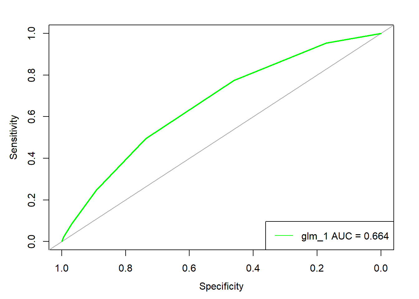
We see that the curve lies over the diagonal but it does not have a strong tendency to touch the upper left corner. A more complex model may perform better but would involve a larger amount of predictors so naturally the question of variable selection will come up.
12.7 Variable selection
Many articles and book chapters have been written on the topic of variable selection (feature selection) and some authors believe it is one of, if not the most, important topic in model buidling. A few good resources giving an overview, can be found below:
- An Introduction to Statistical Learning - Chapter 6: Linear Model Selection and Regularization
- An Introduction to Variable and Feature Selection
- Variable selection methods in regression: Ignorable problem, outing notable solution
The different approaches can be categorized as follows:
- subset selection
- best subset selection
- stepwise selection (forward/backward/hybrid)
- shrinkage
- ridge regression (l2-norm)
- lasso (l1-norm)
- dimension reduction
- principal component analysis (PCA)
There are many trade-offs to be made when choosing one approach over the other but the two most important are statistical soundness and computational efficiency. We will not go into further details of variable selection but rather focus on the model building. We thus simply detrmine a predictor space that seems sensible given prior analysis.
Let’s remind ourselves of variables left for modeling.
full_vars <- colnames(train_down)
full_vars
## [1] "term" "int_rate"
## [3] "grade" "emp_length"
## [5] "home_ownership" "annual_inc"
## [7] "verification_status" "issue_d"
## [9] "pymnt_plan" "purpose"
## [11] "addr_state" "dti"
## [13] "delinq_2yrs" "earliest_cr_line"
## [15] "inq_last_6mths" "open_acc"
## [17] "pub_rec" "revol_bal"
## [19] "revol_util" "initial_list_status"
## [21] "out_prncp_inv" "total_rec_late_fee"
## [23] "collection_recovery_fee" "last_pymnt_d"
## [25] "last_pymnt_amnt" "last_credit_pull_d"
## [27] "collections_12_mths_ex_med" "mths_since_last_major_derog"
## [29] "application_type" "acc_now_delinq"
## [31] "tot_coll_amt" "tot_cur_bal"
## [33] "default"We determine a subspace and report which variables we ignore.
model_vars <-
  c("term", "grade", "emp_length", "home_ownership", "annual_inc",
    "purpose", "pymnt_plan", "out_prncp_inv", "delinq_2yrs", "default")

ignored_vars <- dplyr::setdiff(full_vars, model_vars)
ignored_vars
## [1] "int_rate" "verification_status"
## [3] "issue_d" "addr_state"
## [5] "dti" "earliest_cr_line"
## [7] "inq_last_6mths" "open_acc"
## [9] "pub_rec" "revol_bal"
## [11] "revol_util" "initial_list_status"
## [13] "total_rec_late_fee" "collection_recovery_fee"
## [15] "last_pymnt_d" "last_pymnt_amnt"
## [17] "last_credit_pull_d" "collections_12_mths_ex_med"
## [19] "mths_since_last_major_derog" "application_type"
## [21] "acc_now_delinq" "tot_coll_amt"
## [23] "tot_cur_bal"12.8 A more complex logistic model with caret
The interested reader should check the comprehensive caret documentation on how the API works and for modeling in particular read model training and tuning. We only give a high-level overview here.
The caret package has several functions that attempt to streamline the model building and evaluation process. The train function can be used to
- evaluate, using resampling, the effect of model tuning parameters on performance
- choose the “optimal” model across these parameters
- estimate model performance from a training set
First, a specific model must be chosen. User-defined models can also be created. Second, the corresponding model parameters need to be passed to the function call. The workhorse function is caret::train() but an important input is parameter trControl which also allows specifying a particular resampling approach, e.g. k-fold cross-validation (once or repeated), leave-one-out cross-validation and bootstrap (simple estimation or the 632 rule), etc.
12.8.1 trainControl
We will define the controlling parameters in a separate function call to caret::trainControl() and then pass this on to caret::train(trControl = ). This also allows using the control parameters for different models if applicable to those. The function caret::trainControl() generates parameters that further control how models are created. For more details, see The caret package 5.5.4: The trainControl Function.
We perform a 10-fold cross-validation repeated five times and return the class probabilities. Since we are interested in ROC as our performance measure, we need to set summaryFunction = twoClassSummary. If one likes to see a live log of the execution, verboseIter = TRUE provides that. Since we have no tuning parameters for logistic regression, we leave those out for now.
ctrl <-
  trainControl(method = "repeatedcv",
               number = 10,
               repeats = 5,
               classProbs = TRUE,
               summaryFunction = twoClassSummary,
               savePredictions = TRUE,
               verboseIter = FALSE)
12.8.2 train
Finally, we can call caret::train() with specified control parameters. Note that caret is picky about factor values which need to be valid R names. We thus convert the default variable to have values “yes” and “no” rather than “TRUE” and “FALSE” (which when converted to variable names would not be valid as they are reserved keywords). Make sure that the test set is transformed likewise when using the model for prediction as otherwise your factor levels may be different to the training set and the class probabilities thus wrong.
We will skip the complex discussion around variable selection for now and simply determine the “base” variable universe that seems plausible from intuition and prior exploratory analysis. We have removed categorical variables with many unique values (such as zip codes) as they would be mutated to large dummy matrices.
model_glm_2 <-
  train_down %>%
  select(model_vars) %>%
  mutate(default = as.factor(ifelse(default == TRUE, "yes", "no"))) %>%
  filter(complete.cases(.)) %>%
  train(default ~ .,
        data = .,
        method = "glm",
        family = "binomial",
        metric = "ROC",
        trControl = ctrl)
As with the previous model object created via stats::glm(), the final model object created has many methods and attributes for further processing. But we first look at the results/performance on the training set (which should give a fair estimate of the test set performance since we used cross-validation). Note that all reported metrics are interpretable since this is done on the balanced data.
model_glm_2## Generalized Linear Model
##
## 35488 samples
## 9 predictor
## 2 classes: 'no', 'yes'
##
## No pre-processing
## Resampling: Cross-Validated (10 fold, repeated 5 times)
## Summary of sample sizes: 31938, 31938, 31940, 31939, 31940, 31940, ...
## Resampling results:
##
## ROC Sens Spec
## 0.6964721 0.6291356 0.662019We can see that we have improved on the ROCAUC (~ 70%) but got worse for sensitivity compared to the first, simpler model. Looking at the predictors, we also see how the model created dummies to encode categorical variables.
attributes(model_glm_2)## $names
## [1] "method" "modelInfo" "modelType" "results"
## [5] "pred" "bestTune" "call" "dots"
## [9] "metric" "control" "finalModel" "preProcess"
## [13] "trainingData" "resample" "resampledCM" "perfNames"
## [17] "maximize" "yLimits" "times" "levels"
## [21] "terms" "coefnames" "contrasts" "xlevels"
##
## $class
## [1] "train" "train.formula"summary(model_glm_2)##
## Call:
## NULL
##
## Deviance Residuals:
## Min 1Q Median 3Q Max
## -2.3163 -1.0774 -0.2782 1.0635 5.6347
##
## Coefficients:
## Estimate Std. Error z value
## (Intercept) -1.7381657126 0.1420955332 -12.232
## termX60.months -0.5453038253 0.0298754606 -18.253
## gradeB 0.8159277950 0.0461745543 17.671
## gradeC 1.3693629935 0.0459015145 29.833
## gradeD 1.7227789216 0.0490499846 35.123
## gradeE 2.0514999392 0.0562719050 36.457
## gradeF 2.3642399559 0.0741417266 31.888
## gradeG 2.8775473195 0.1315002573 21.882
## emp_lengthX..1.year 0.0719719375 0.0634309986 1.135
## emp_lengthX1.year -0.0231801001 0.0663542839 -0.349
## emp_lengthX10..years -0.1447186450 0.0541082748 -2.675
## emp_lengthX2.years -0.0155518922 0.0628511985 -0.247
## emp_lengthX3.years 0.0019357572 0.0640494674 0.030
## emp_lengthX4.years -0.0416200714 0.0681959839 -0.610
## emp_lengthX5.years -0.1208526942 0.0671199278 -1.801
## emp_lengthX6.years 0.0685014427 0.0713774190 0.960
## emp_lengthX7.years 0.0169740882 0.0708191548 0.240
## emp_lengthX8.years -0.0231357344 0.0711988793 -0.325
## emp_lengthX9.years -0.0454158473 0.0751319778 -0.604
## home_ownershipNONE -0.5795772695 1.3066383779 -0.444
## home_ownershipOTHER 12.3599134059 91.3562921237 0.135
## home_ownershipOWN 0.1059366445 0.0397823985 2.663
## home_ownershipRENT 0.1738380528 0.0253881630 6.847
## annual_inc -0.0000018620 0.0000002708 -6.875
## purposecredit_card 0.0940714394 0.1290711042 0.729
## purposedebt_consolidation 0.1957294997 0.1273405178 1.537
## purposeeducational 1.4894997798 0.4601526184 3.237
## purposehome_improvement 0.2605554222 0.1355011685 1.923
## purposehouse 0.0010870105 0.2087251602 0.005
## purposemajor_purchase 0.1111783795 0.1507309963 0.738
## purposemedical 0.1525955150 0.1664861916 0.917
## purposemoving 0.4431876570 0.1857656345 2.386
## purposeother 0.0979564862 0.1356860122 0.722
## purposerenewable_energy 0.0910160004 0.4132422786 0.220
## purposesmall_business 0.2405034075 0.1572708880 1.529
## purposevacation 0.1203054032 0.1926193435 0.625
## purposewedding -0.4075063208 0.3202319627 -1.273
## pymnt_plany 11.9809020840 154.7613613910 0.077
## out_prncp_inv 0.0000520918 0.0000017015 30.614
## delinq_2yrs 0.0865718494 0.0125320528 6.908
## Pr(>|z|)
## (Intercept) < 0.0000000000000002 ***
## termX60.months < 0.0000000000000002 ***
## gradeB < 0.0000000000000002 ***
## gradeC < 0.0000000000000002 ***
## gradeD < 0.0000000000000002 ***
## gradeE < 0.0000000000000002 ***
## gradeF < 0.0000000000000002 ***
## gradeG < 0.0000000000000002 ***
## emp_lengthX..1.year 0.25652
## emp_lengthX1.year 0.72684
## emp_lengthX10..years 0.00748 **
## emp_lengthX2.years 0.80457
## emp_lengthX3.years 0.97589
## emp_lengthX4.years 0.54166
## emp_lengthX5.years 0.07177 .
## emp_lengthX6.years 0.33720
## emp_lengthX7.years 0.81058
## emp_lengthX8.years 0.74522
## emp_lengthX9.years 0.54552
## home_ownershipNONE 0.65736
## home_ownershipOTHER 0.89238
## home_ownershipOWN 0.00775 **
## home_ownershipRENT 0.00000000000753 ***
## annual_inc 0.00000000000621 ***
## purposecredit_card 0.46610
## purposedebt_consolidation 0.12428
## purposeeducational 0.00121 **
## purposehome_improvement 0.05449 .
## purposehouse 0.99584
## purposemajor_purchase 0.46076
## purposemedical 0.35937
## purposemoving 0.01705 *
## purposeother 0.47033
## purposerenewable_energy 0.82568
## purposesmall_business 0.12621
## purposevacation 0.53225
## purposewedding 0.20318
## pymnt_plany 0.93829
## out_prncp_inv < 0.0000000000000002 ***
## delinq_2yrs 0.00000000000491 ***
## ---
## Signif. codes: 0 '***' 0.001 '**' 0.01 '*' 0.05 '.' 0.1 ' ' 1
##
## (Dispersion parameter for binomial family taken to be 1)
##
## Null deviance: 49197 on 35487 degrees of freedom
## Residual deviance: 44806 on 35448 degrees of freedom
## AIC: 44886
##
## Number of Fisher Scoring iterations: 11predictors(model_glm_2)## [1] "termX60.months" "gradeB"
## [3] "gradeC" "gradeD"
## [5] "gradeE" "gradeF"
## [7] "gradeG" "emp_lengthX..1.year"
## [9] "emp_lengthX1.year" "emp_lengthX10..years"
## [11] "emp_lengthX2.years" "emp_lengthX3.years"
## [13] "emp_lengthX4.years" "emp_lengthX5.years"
## [15] "emp_lengthX6.years" "emp_lengthX7.years"
## [17] "emp_lengthX8.years" "emp_lengthX9.years"
## [19] "home_ownershipNONE" "home_ownershipOTHER"
## [21] "home_ownershipOWN" "home_ownershipRENT"
## [23] "annual_inc" "purposecredit_card"
## [25] "purposedebt_consolidation" "purposeeducational"
## [27] "purposehome_improvement" "purposehouse"
## [29] "purposemajor_purchase" "purposemedical"
## [31] "purposemoving" "purposeother"
## [33] "purposerenewable_energy" "purposesmall_business"
## [35] "purposevacation" "purposewedding"
## [37] "pymnt_plany" "out_prncp_inv"
## [39] "delinq_2yrs"We can also look at the variable importance with caret::varImp(). For linear models, the absolute value of the t-statistic for each model parameter is used.
varImp(model_glm_2)## glm variable importance
##
## only 20 most important variables shown (out of 39)
##
## Overall
## gradeE 100.000
## gradeD 96.340
## gradeF 87.466
## out_prncp_inv 83.972
## gradeC 81.827
## gradeG 60.017
## termX60.months 50.059
## gradeB 48.462
## delinq_2yrs 18.937
## annual_inc 18.846
## home_ownershipRENT 18.770
## purposeeducational 8.866
## emp_lengthX10..years 7.323
## home_ownershipOWN 7.291
## purposemoving 6.531
## purposehome_improvement 5.261
## emp_lengthX5.years 4.925
## purposedebt_consolidation 4.202
## purposesmall_business 4.181
## purposewedding 3.477plot(varImp(model_glm_2))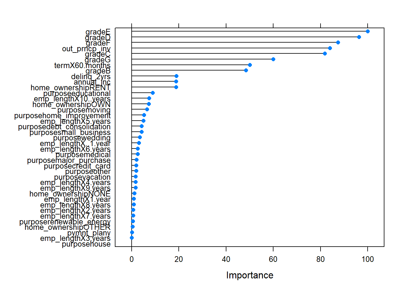
Finally, we use the model to predict the test set classes. Again, we need to be aware of any pre-processing required such as mutations or treatment of missing values.
model_glm_2_pred <-
  predict(model_glm_2,
          newdata = test %>%
            select(model_vars) %>%
            mutate(default = as.factor(ifelse(default == TRUE,
                                              "yes", "no"))) %>%
            filter(complete.cases(.)),
          type = "prob")

head(model_glm_2_pred, 3)
## no yes
## 1 0.7041954 0.2958046
## 2 0.8783103 0.1216897
## 3 0.6509819 0.3490181Note that caret::predict.train returns the probabilties for all outcomes i.e. in our binary case for yes and no. We repeat the analysis from earlier and see how the new model performs.
caret::confusionMatrix(
  data = ifelse(model_glm_2_pred[, "yes"] > 0.5, "yes", "no"),
  reference = as.factor(ifelse(test[complete.cases(test[, model_vars]),
                                    "default"] == TRUE, "yes", "no")),
  positive = "yes")
## Confusion Matrix and Statistics
##
## Reference
## Prediction no yes
## no 109156 1482
## yes 63876 2953
##
## Accuracy : 0.6317
## 95% CI : (0.6295, 0.634)
## No Information Rate : 0.975
## P-Value [Acc > NIR] : 1
##
## Kappa : 0.0378
## Mcnemar's Test P-Value : <0.0000000000000002
##
## Sensitivity : 0.66584
## Specificity : 0.63084
## Pos Pred Value : 0.04419
## Neg Pred Value : 0.98660
## Prevalence : 0.02499
## Detection Rate : 0.01664
## Detection Prevalence : 0.37657
## Balanced Accuracy : 0.64834
##
## 'Positive' Class : yes
## Again we build an ROC object.
temp <- as.factor(ifelse(test[complete.cases(test[, model_vars]),
                                             "default"] == TRUE, "yes", "no"))

roc_glm_2 <-
  pROC::roc(response = temp,
            predictor = model_glm_2_pred[, "yes"])

roc_glm_2
##
## Call:
## roc.default(response = temp, predictor = model_glm_2_pred[, "yes"])
##
## Data: model_glm_2_pred[, "yes"] in 173032 controls (temp no) < 4435 cases (temp yes).
## Area under the curve: 0.6995#data = as.data.frame(unclass(train[complete.cases(train), ]))The ROCAUC of ~ 70% is nearly the same as for the cross-validated training set. We plot the curve comparing it against the ROC from the simple model.
pROC::plot.roc(x = roc_glm_1, legacy.axes = FALSE, xlim = c(1, 0), asp = NA,
               col = "green")

pROC::plot.roc(x = roc_glm_2, legacy.axes = FALSE, xlim = c(1, 0), asp = NA,
               add = TRUE, col = "blue")

legend(x = "bottomright", legend=c("glm_1 AUC = 0.664", "glm_2 AUC = 0.7"),
       col = c("green", "blue"), lty = 1, cex = 1.0)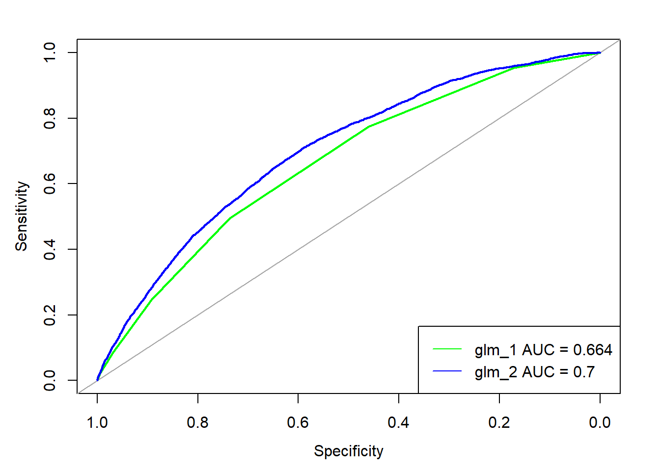
We can see that the more complex model has a better ROC above the simple model.
12.9 A note on computational efficiency (parallelization via cluster)
Some models (and their tuning parameter calibration via resampling) will require significant computational resources both in terms of memory and CPUs. There are a few ways to increase computational efficiency which can be roughly divided into
- decrease training set (without loosing information)
- compute on several cores (parallelization via cluster)
- shift matrix computations to GPU (e.g. via CUDA)
- use compute instances from cloud offerings such as Amazon Web Services, googleCloud or Microsoft Azure
We will only look at parallelization here as it is supported by R and caret out of the box. For details, see The caret package 9: Parallel Processing, caret ml parallel and HOME of the R parallel WIKI! by Tobias Kind. There are a couple of libraries supporting parallel processing in R but one should be aware of the support for different operating systems. On Windows, one should use doParallel which is a parallel backend for the foreach package. Note that the multicore functionality only runs tasks on a single computer, not a cluster of computers. However, you can use the snow functionality to execute on a cluster, using Unix-like operating systems, Windows, or even a combination. It is pointless to use doParallel and parallel on a machine with only one processor with a single core. To get a speed improvement, it must run on a machine with multiple processors, multiple cores, or both. Remember: unless doParallel::registerDoParallel() is called, foreach will not run in parallel. Simply loading the doParallel package is not enough. Note that we can set the parameter caret::trainControl(allowParallel = TRUE) but it is actually the default setting, i.e. caret::train() will automatically run in parallel if it detects a registerd cluster, irrespective of library is used to build it.
To illustrate efficiency gains, we will benchmark an example model training using the previous glm model. We use library (and function with same name) microbenchmark and define to execute the operation several times (to get a stable time estimate) via parameter times. Note that parallizing usually means creating copies of the original data for each worker (core) which requires according memory. Since we only want to illustrate the logic here, we downsize the training data to avoid failures due to insufficient memory.
benchmark_train_data <-
  train_down[seq(1, nrow(train_down), 2), model_vars] %>%
  mutate(default = as.factor(ifelse(default == TRUE, "yes", "no"))) %>%
  filter(complete.cases(.))
format(utils::object.size(benchmark_train_data), units = "Mb")
## [1] "1.3 Mb"We see the data has ~ 1 Mb in size.
ctrl <-
  trainControl(method = "repeatedcv",
               number = 10,
               repeats = 5,
               classProbs = TRUE,
               summaryFunction = twoClassSummary,
               verboseIter = FALSE,
               allowParallel = TRUE) #default

library(microbenchmark)

glm_nopar <-
  microbenchmark(glm_nopar =
      train(default ~ .,
            data = benchmark_train_data,
            method = "glm",
            family = "binomial",
            metric = "ROC",
            trControl = ctrl),
    times = 5
    )
## Warning in predict.lm(object, newdata, se.fit, scale = 1, type =
## ifelse(type == : prediction from a rank-deficient fit may be misleading
## Warning in predict.lm(object, newdata, se.fit, scale = 1, type =
## ifelse(type == : prediction from a rank-deficient fit may be misleading
## Warning in predict.lm(object, newdata, se.fit, scale = 1, type =
## ifelse(type == : prediction from a rank-deficient fit may be misleading
## Warning in predict.lm(object, newdata, se.fit, scale = 1, type =
## ifelse(type == : prediction from a rank-deficient fit may be misleading
## Warning in predict.lm(object, newdata, se.fit, scale = 1, type =
## ifelse(type == : prediction from a rank-deficient fit may be misleading
## Warning in predict.lm(object, newdata, se.fit, scale = 1, type =
## ifelse(type == : prediction from a rank-deficient fit may be misleading
## Warning in predict.lm(object, newdata, se.fit, scale = 1, type =
## ifelse(type == : prediction from a rank-deficient fit may be misleading
## Warning in predict.lm(object, newdata, se.fit, scale = 1, type =
## ifelse(type == : prediction from a rank-deficient fit may be misleading
## Warning in predict.lm(object, newdata, se.fit, scale = 1, type =
## ifelse(type == : prediction from a rank-deficient fit may be misleading
## Warning in predict.lm(object, newdata, se.fit, scale = 1, type =
## ifelse(type == : prediction from a rank-deficient fit may be misleadingWe can look at the resulting run time.
glm_nopar## Unit: seconds
## expr min lq mean median uq max neval
## glm_nopar 27.51427 27.90744 28.27665 28.38591 28.71571 28.8599 5Now, we will setup a cluster of cores and repeat the benchmarking. We use parallel::detectCores() to establish how many cores are available and use some amount smaller 100% of cores to leave some resources for the system. Usually, we would write a log of the distributed calculation via parallel::makeCluster(outfile = ). It will be opened in append mode as all workers write to it. However, we found issues with running parallel::makeCluster(outfile = ) so we simply run the cluster directly from registerDoParallel() which has no option to define a log file.
# doParallel would also load parallel
library(parallel)
library(doParallel)
## Warning: package 'doParallel' was built under R version 3.4.2## Loading required package: foreach##
## Attaching package: 'foreach'## The following objects are masked from 'package:purrr':
##
## accumulate, when## Loading required package: iteratorscores_2_use <- floor(0.8 * detectCores())
# cl <- makeCluster(cores_2_use, outfile = "./logs/parallel_log.txt")
# registerDoParallel(cl, cores_2_use)
registerDoParallel(cores = cores_2_use)
getDoParWorkers()## [1] 6We can inspect the open connections via base::showConnections().
knitr::kable(base::showConnections())| description | class | mode | text | isopen | can read | can write | |
|---|---|---|---|---|---|---|---|
| 4 | output | textConnection | wr | text | opened | no | yes |
| 5 | <-eclipse:11076 | sockconn | a+b | binary | opened | yes | yes |
| 6 | <-eclipse:11076 | sockconn | a+b | binary | opened | yes | yes |
| 7 | <-eclipse:11076 | sockconn | a+b | binary | opened | yes | yes |
| 8 | <-eclipse:11076 | sockconn | a+b | binary | opened | yes | yes |
| 9 | <-eclipse:11076 | sockconn | a+b | binary | opened | yes | yes |
| 10 | <-eclipse:11076 | sockconn | a+b | binary | opened | yes | yes |
Now we tried running in parallel but the setup may produce an error on Windows.
Error in e$fun(obj, substitute(ex), parent.frame(), e$data) : unable to find variable "optimismBoot"
This seems to be a bug as noted in SO question Caret train function - unable to find variable “optimismBoot”. The bug seems to be solved in caret development version which can be installed from GitHub via devtools::install_github('topepo/caret/pkg/caret') (note that building caret from source requires RBuildTools which are part of RTools which need to be installed separately, e.g. from Building R for Windows - RStudio may manage the install for you). The issue is also tracked on GitHub under optimismBoot error #706 and may already be resolved in the caret version you are using.
We do not run the install of the development version here again but you should in case you do not have it and wish to test the parallel execution. Before you do, make sure to close the cluster with below code (not executed now as we continue).
parallel::stopCluster(cl)
foreach::registerDoSEQ()
glm_par <-
microbenchmark(glm_par =
train(default ~ .,
data = benchmark_train_data,
method = "glm",
family = "binomial",
metric = "ROC",
trControl = ctrl),
times = 5
)We make sure to stop the cluster and force R back to sequential execution by using foreach::registerDoSEQ(). In case you used the setup via parallel::makeCluster(), you need to call parallel::stopCluster() first. Otherwise, memory and CPU may be occupied with legacy clusters.
#parallel::stopCluster(cl)
foreach::registerDoSEQ()
Note that we ran into issues when using too much system resources on a Windows 7 workstation as documented in the SO question caret train binary glm fails on parallel cluster via doParallel. Below error was produced.
Error in serialize(data, node$con) : error writing to connection
However, on a Windows 10 machine with fewer cores and development version of caret the issue could not be reproduced.
We have also tried running caret::train() parallel on Linux (Ubuntu) via the doMC library and found that below setting runs just fine and also faster than a sequential execution. We only include the code here for info without execution.
library(doMC)

cores_2_use <- floor(0.8 * parallel::detectCores())
registerDoMC(cores_2_use)

microbenchmark(
  glm_par =
    train(y ~ .,
          data = df,
          method = "glm",
          family = "binomial",
          metric = "ROC",
          trControl = ctrl),
  times = 5)
Finally, let’s compare parallel versus non-parallel execution time. We can see that the parallel setup performed significantly better but we would have expected even more as we are using a multiple of the one-core setup.
glm_nopar## Unit: seconds
## expr min lq mean median uq max neval
## glm_nopar 27.51427 27.90744 28.27665 28.38591 28.71571 28.8599 5glm_par## Unit: seconds
## expr min lq mean median uq max neval
## glm_par 13.65229 13.79392 17.34424 13.8397 13.89238 31.54293 512.10 A note on tuning parameters in caret
When it comes to more complex models in general, often tuning parameters can be used to improve the model. There are different ways to provide the range of parameters to take. In particular, one may use
- pre-defined number (e.g. if domain knowledge already provides and idea)
- use grid search (default in
caret::train()) - use random search
In general, the more tuning parameters are available, the higher the computational cost of selecting them. We will show some applications of options below. For further information, see The caret package 5: Model Training and Tuning
12.11 Trees
Trees stratify or segment the predictor space into a number of simple regions. In order to make a prediction for a given observation, we typically use the mean or the mode of the training observations in the region to which it belongs. Trees are easy to interpret and built but as pointed out in “An Introduction to Statistical Learning” they may not compete with the best supervised learning approaches:
Tree-based methods are simple and useful for interpretation. However, they typically are not competitive with the best supervised learning approaches, such as those seen in Chapters 6 and 7, in terms of prediction accuracy. Hence in this chapter we also introduce bagging, random forests, and boosting. Each of these approaches involves producing multiple trees which are then combined to yield a single consensus prediction. We will see that combining a large number of trees can often result in dramatic improvements in prediction accuracy, at the expense of some loss in interpretation.
Following this guidance, we will also look into some alternatives / enhancements of the basic tree model used in CART. Some further resources on trees are found in
- An Introduction to Statistical Learning
- A Complete Tutorial on Tree Based Modeling from Scratch (in R & Python)
As usual, there are many ways to implement tree models in R but we will stay within the caret package and use the API that was already explained earlier.
12.11.1 Simple tree using CART via rpart in caret
We start by building a simple tree using the CART method via rpart in caret. Note that caret may not offer the full set of features that are available when using the rpart library directly but it should suffice for our illustration. For more details, see rpart on CRAN and in particular An Introduction to Recursive Partitioning Using the RPART Routines for some background.
We define our control and train functions as before and look at the results.
ctrl <-
  trainControl(method = "repeatedcv",
               number = 10,
               repeats = 5,
               classProbs = TRUE,
               summaryFunction = twoClassSummary,
               verboseIter = FALSE,
               allowParallel = TRUE)

# library(rpart)

model_rpart <-
  train_down %>%
  select(model_vars) %>%
  mutate(default = as.factor(ifelse(default == TRUE, "yes", "no"))) %>%
  filter(complete.cases(.)) %>%
  train(default ~ .,
        data = .,
        method = 'rpart',
        metric = "ROC",
        preProc = c("center", "scale"),
        trControl = ctrl)
## Warning in preProcess.default(thresh = 0.95, k = 5, freqCut = 19, uniqueCut
## = 10, : These variables have zero variances: home_ownershipNONEmodel_rpart## CART
##
## 35488 samples
## 9 predictor
## 2 classes: 'no', 'yes'
##
## Pre-processing: centered (39), scaled (39)
## Resampling: Cross-Validated (10 fold, repeated 5 times)
## Summary of sample sizes: 31939, 31938, 31940, 31939, 31940, 31939, ...
## Resampling results across tuning parameters:
##
## cp ROC Sens Spec
## 0.01445641 0.7018554 0.5572830 0.7674466
## 0.03111086 0.6461547 0.3900115 0.8799842
## 0.26027166 0.5707699 0.6019078 0.5396320
##
## ROC was used to select the optimal model using the largest value.
## The final value used for the model was cp = 0.01445641.We see that ROCAUC is ~ 70% for the best model iteration but sensitivity is worse than in some previous models. caret stepped through some complexity parameters (cp) and printed results for them. We can look at cp visually for the different values. In fact, under caret this is the only tuning parameter available for method = rpart.
ggplot(model_rpart)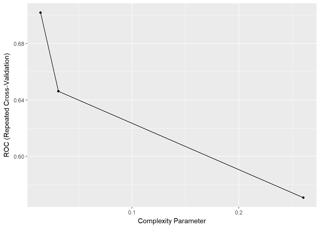
We can also visualize the final tree by accessing the finalModel element from the caret::train() model object. We have to add the text manually to the plot via graphics::text(). We use a larger margin to have enough space for the text.
plot(model_rpart$finalModel, uniform = TRUE, margin = 0.2)
graphics::text(model_rpart$finalModel)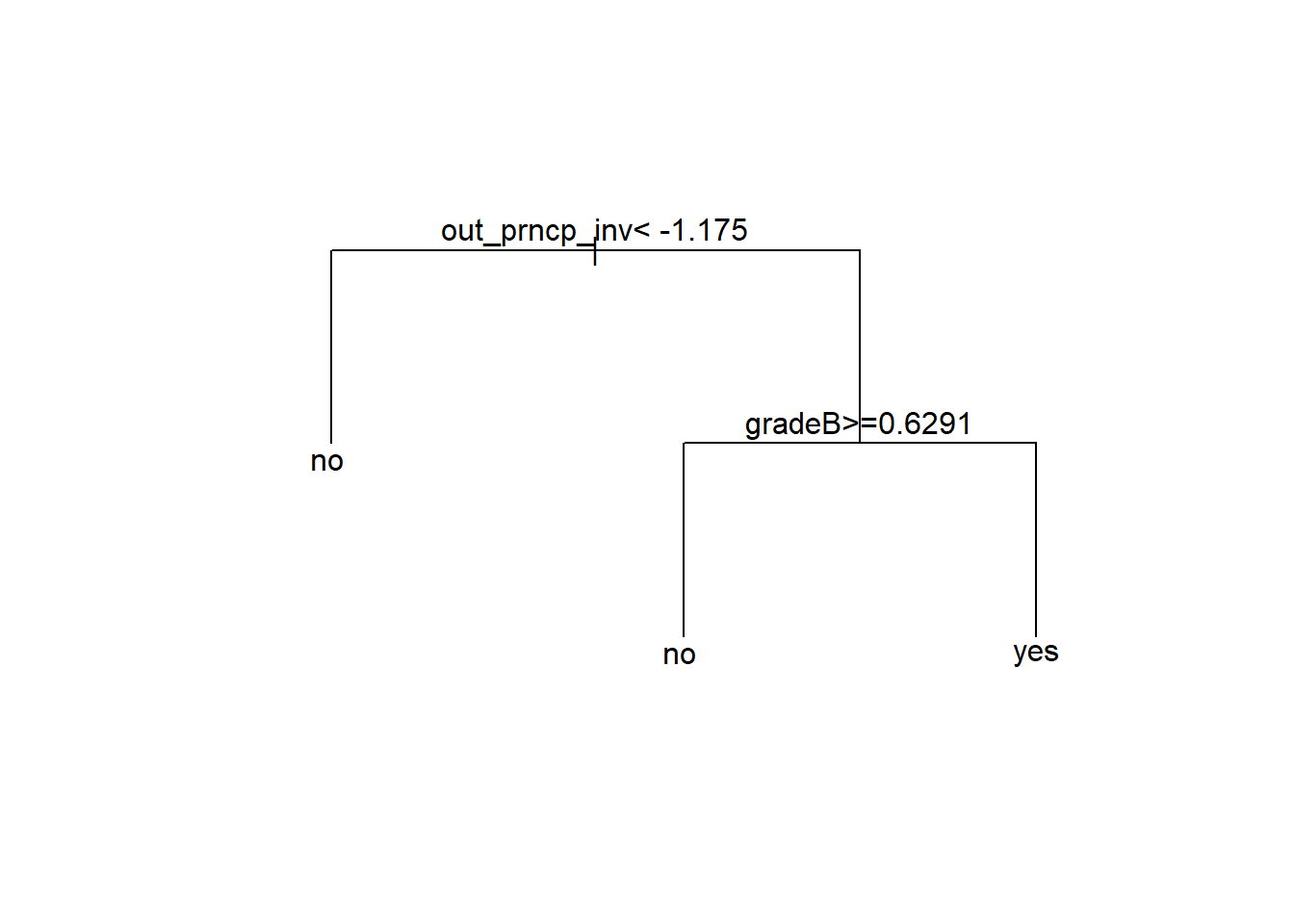
Apparently, there are only two splits, for out_prncp_inv and gradeB.
Rather than using the default grid search for choosing the tuning parameter cp, we could use random search (as mentioned earlier). For a theoretical background on why this might be useful, see e.g. Random Search for Hyper-Parameter Optimization. We implement random search via the parameter caret::trainControl(search = "random").
ctrl <-
  trainControl(method = "repeatedcv",
               number = 10,
               repeats = 5,
               classProbs = TRUE,
               summaryFunction = twoClassSummary,
               verboseIter = FALSE,
               allowParallel = TRUE,
               search = "random")

model_rpart <-
  train_down %>%
  select(model_vars) %>%
  mutate(default = as.factor(ifelse(default == TRUE, "yes", "no"))) %>%
  filter(complete.cases(.)) %>%
  train(default ~ .,
        data = .,
        method = 'rpart',
        metric = "ROC",
        preProc = c("center", "scale"),
        trControl = ctrl)

model_rpart
## CART
##
## 35488 samples
## 9 predictor
## 2 classes: 'no', 'yes'
##
## Pre-processing: centered (39), scaled (39)
## Resampling: Cross-Validated (10 fold, repeated 5 times)
## Summary of sample sizes: 31939, 31940, 31940, 31938, 31940, 31940, ...
## Resampling results across tuning parameters:
##
## cp ROC Sens Spec
## 0.0002254410 0.7418953 0.5806143 0.7904981
## 0.0002536211 0.7433551 0.5725220 0.8003501
## 0.0005072423 0.7462419 0.5532501 0.8225663
##
## ROC was used to select the optimal model using the largest value.
## The final value used for the model was cp = 0.0005072423.We can see that ROCAUC went up to ~ 74% and sensitivity also increased somewhat with the random search cp parameterization which ended up using a value much smaller than grid search. We again visualize the tree to see how it changed.
plot(model_rpart$finalModel, uniform = TRUE, margin = 0.1)
graphics::text(model_rpart$finalModel, cex = 0.5)
Clearly the model has become more complex which was expected given that its ROCAUC went up. As before, we will predict test outcome with the final model.
model_rpart_pred <-
  predict(model_rpart,
          newdata = test %>%
            select(model_vars) %>%
            mutate(default = as.factor(ifelse(default == TRUE,
                                              "yes", "no"))) %>%
            filter(complete.cases(.)),
          type = "prob")

caret::confusionMatrix(
  data = ifelse(model_rpart_pred[, "yes"] > 0.5, "yes", "no"),
  reference = as.factor(ifelse(test[complete.cases(test[, model_vars]),
                                    "default"] == TRUE, "yes", "no")),
  positive = "yes")
## Confusion Matrix and Statistics
##
## Reference
## Prediction no yes
## no 91226 682
## yes 81806 3753
##
## Accuracy : 0.5352
## 95% CI : (0.5329, 0.5375)
## No Information Rate : 0.975
## P-Value [Acc > NIR] : 1
##
## Kappa : 0.0377
## Mcnemar's Test P-Value : <0.0000000000000002
##
## Sensitivity : 0.84622
## Specificity : 0.52722
## Pos Pred Value : 0.04386
## Neg Pred Value : 0.99258
## Prevalence : 0.02499
## Detection Rate : 0.02115
## Detection Prevalence : 0.48211
## Balanced Accuracy : 0.68672
##
## 'Positive' Class : yes
## Compute ROC.
roc_rpart <-
  pROC::roc(response = temp,
            predictor = model_rpart_pred[, "yes"])

roc_rpart
##
## Call:
## roc.default(response = temp, predictor = model_rpart_pred[, "yes"])
##
## Data: model_rpart_pred[, "yes"] in 173032 controls (temp no) < 4435 cases (temp yes).
## Area under the curve: 0.7463The ROCAUC is ~74% which is nearly the same as for cross-validated training set. We plot the curve comparing it against the ROC from earlier models.
pROC::plot.roc(x = roc_glm_1, legacy.axes = FALSE, xlim = c(1, 0), asp = NA,
               col = "green")

pROC::plot.roc(x = roc_glm_2, legacy.axes = FALSE, xlim = c(1, 0), asp = NA,
               add = TRUE, col = "blue")

pROC::plot.roc(x = roc_rpart, legacy.axes = FALSE, xlim = c(1, 0), asp = NA,
               add = TRUE, col = "orange")


legend(x = "bottomright", legend=c("glm_1 AUC = 0.664", "glm_2 AUC = 0.7",
                                   "rpart AUC = 0.74"),
       col = c("green", "blue", "orange"), lty = 1, cex = 1.0)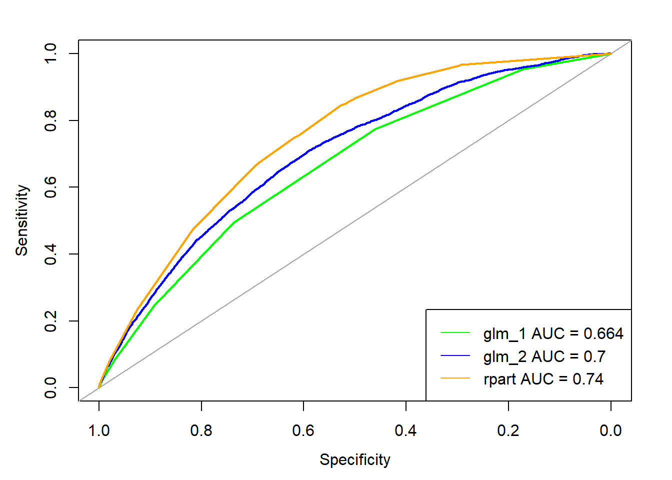
12.11.2 Random forest via randomForest in caret
For random forests, the library randomForest is used. Tuning parameter is mtry which is the number of variables randomly sampled as candidates at each split. For computationally reasons, we limit the number of trees via caret::trainControl(ntree)), the number of folds via caret::trainControl(number)) and the resampling iterations via caret::trainControl(repeats)).
# library(randomForest)

ctrl <-
  trainControl(method = "repeatedcv",
               number = 5,
               repeats = 1,
               classProbs = TRUE,
               summaryFunction = twoClassSummary,
               verboseIter = FALSE,
               allowParallel = TRUE)

model_rf <-
  train_down %>%
  select(model_vars) %>%
  mutate(default = as.factor(ifelse(default == TRUE, "yes", "no"))) %>%
  filter(complete.cases(.)) %>%
  train(default ~ .,
        data = .,
        method = 'rf',
        ntree = 10,
        metric = "ROC",
        preProc = c("center", "scale"),
        trControl = ctrl)

model_rf
## Random Forest
##
## 35488 samples
## 9 predictor
## 2 classes: 'no', 'yes'
##
## Pre-processing: centered (39), scaled (39)
## Resampling: Cross-Validated (5 fold, repeated 1 times)
## Summary of sample sizes: 28391, 28390, 28390, 28391, 28390
## Resampling results across tuning parameters:
##
## mtry ROC Sens Spec
## 2 0.6877044 0.5636517 0.7134646
## 20 0.7041407 0.6133559 0.6806064
## 39 0.6982071 0.6123415 0.6655027
##
## ROC was used to select the optimal model using the largest value.
## The final value used for the model was mtry = 20.We can see that ROCAUC is ~ 70% at mtry = 20. We again visualize but since it is a combination of many trees, the plot will look different.
plot(model_rf$finalModel)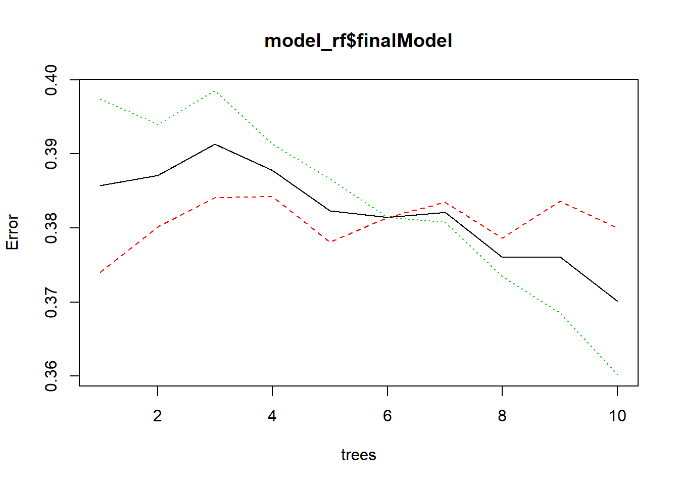
The error would most likely go further down if we had allowed more trees.
model_rf_pred <-
  predict(model_rf,
          newdata = test %>%
            select(model_vars) %>%
            mutate(default = as.factor(ifelse(default == TRUE,
                                              "yes", "no"))) %>%
            filter(complete.cases(.)),
          type = "prob")

caret::confusionMatrix(
  data = ifelse(model_rf_pred[, "yes"] > 0.5, "yes", "no"),
  reference = as.factor(ifelse(test[complete.cases(test[, model_vars]),
                                    "default"] == TRUE, "yes", "no")),
  positive = "yes")
## Confusion Matrix and Statistics
##
## Reference
## Prediction no yes
## no 114693 1723
## yes 58339 2712
##
## Accuracy : 0.6616
## 95% CI : (0.6594, 0.6638)
## No Information Rate : 0.975
## P-Value [Acc > NIR] : 1
##
## Kappa : 0.038
## Mcnemar's Test P-Value : <0.0000000000000002
##
## Sensitivity : 0.61150
## Specificity : 0.66284
## Pos Pred Value : 0.04442
## Neg Pred Value : 0.98520
## Prevalence : 0.02499
## Detection Rate : 0.01528
## Detection Prevalence : 0.34401
## Balanced Accuracy : 0.63717
##
## 'Positive' Class : yes
## Compute ROC.
roc_rf <-
  pROC::roc(response = temp,
            predictor = model_rf_pred[, "yes"])

roc_rf
##
## Call:
## roc.default(response = temp, predictor = model_rf_pred[, "yes"])
##
## Data: model_rf_pred[, "yes"] in 173032 controls (temp no) < 4435 cases (temp yes).
## Area under the curve: 0.7021As the ROCAUC is not better than before, we will not plot it against earlier models.
12.11.3 Stochastic Gradient Boosting via gbm in caret
For Stochastic Gradient Boosting, the library gbm is used. Tuning parameters are
- n.trees: total number of trees to fit
- interaction.depth: maximum depth of variable interactions
- shrinkage: shrinkage parameter applied to each tree in the expansion
- n.minobsinnode: minimum number of observations in the trees terminal nodes
For some background, see e.g.
- Stochastic Gradient Boosting, Jerome Friedman
- A Gentle Introduction to the Gradient Boosting Algorithm for Machine Learning
# library(gbm)

ctrl <-
  trainControl(method = "repeatedcv",
               number = 5,
               repeats = 1,
               classProbs = TRUE,
               summaryFunction = twoClassSummary,
               verboseIter = FALSE,
               allowParallel = TRUE)

model_gbm_1 <-
   train_down %>%
   select(model_vars) %>%
   mutate(default = as.factor(ifelse(default == TRUE, "yes", "no"))) %>%
   filter(complete.cases(.)) %>%
   train(default ~ .,
         data = .,
         method = "gbm",
         metric = "ROC",
         trControl = ctrl,
         preProc = c("center", "scale"),
         ## This last option is actually one
         ## for gbm() that passes through
         verbose = FALSE)

model_gbm_1
## Stochastic Gradient Boosting
##
## 35488 samples
## 9 predictor
## 2 classes: 'no', 'yes'
##
## Pre-processing: centered (39), scaled (39)
## Resampling: Cross-Validated (5 fold, repeated 1 times)
## Summary of sample sizes: 28390, 28391, 28390, 28390, 28391
## Resampling results across tuning parameters:
##
## interaction.depth n.trees ROC Sens Spec
## 1 50 0.7218075 0.4989575 0.7923127
## 1 100 0.7347236 0.5438152 0.7776594
## 1 150 0.7376056 0.5922232 0.7565241
## 2 50 0.7351958 0.5467456 0.7754611
## 2 100 0.7416798 0.6105945 0.7484081
## 2 150 0.7480446 0.6190476 0.7499302
## 3 50 0.7387262 0.6076078 0.7507755
## 3 100 0.7488759 0.6164553 0.7538746
## 3 150 0.7515752 0.6082840 0.7630048
##
## Tuning parameter 'shrinkage' was held constant at a value of 0.1
##
## Tuning parameter 'n.minobsinnode' was held constant at a value of 10
## ROC was used to select the optimal model using the largest value.
## The final values used for the model were n.trees = 150,
## interaction.depth = 3, shrinkage = 0.1 and n.minobsinnode = 10.Plotting the boosting iterations.
ggplot(model_gbm_1)## Warning: Ignoring unknown aesthetics: shape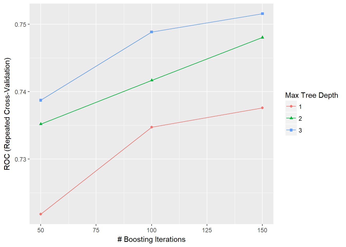
Predict.
model_gbm_1_pred <-
  predict(model_gbm_1,
          newdata = test %>%
            select(model_vars) %>%
            mutate(default = as.factor(ifelse(default == TRUE,
                                              "yes", "no"))) %>%
            filter(complete.cases(.)),
          type = "prob")

caret::confusionMatrix(
  data = ifelse(model_gbm_1_pred[, "yes"] > 0.5, "yes", "no"),
  reference = as.factor(ifelse(test[complete.cases(test[, model_vars]),
                                    "default"] == TRUE, "yes", "no")),
  positive = "yes")
## Confusion Matrix and Statistics
##
## Reference
## Prediction no yes
## no 104238 1033
## yes 68794 3402
##
## Accuracy : 0.6065
## 95% CI : (0.6043, 0.6088)
## No Information Rate : 0.975
## P-Value [Acc > NIR] : 1
##
## Kappa : 0.0438
## Mcnemar's Test P-Value : <0.0000000000000002
##
## Sensitivity : 0.76708
## Specificity : 0.60242
## Pos Pred Value : 0.04712
## Neg Pred Value : 0.99019
## Prevalence : 0.02499
## Detection Rate : 0.01917
## Detection Prevalence : 0.40681
## Balanced Accuracy : 0.68475
##
## 'Positive' Class : yes
## roc_gbm_1 <-
pROC::roc(response = temp,
predictor = model_gbm_1_pred[, "yes"])
roc_gbm_1##
## Call:
## roc.default(response = temp, predictor = model_gbm_1_pred[, "yes"])
##
## Data: model_gbm_1_pred[, "yes"] in 173032 controls (temp no) < 4435 cases (temp yes).
## Area under the curve: 0.7516The ROCAUC is ~75% which is nearly the same as for cross-validated training set. We plot the curve comparing it against the ROC from the simple model.
pROC::plot.roc(x = roc_glm_1, legacy.axes = FALSE, xlim = c(1, 0), asp = NA,
               col = "green")

pROC::plot.roc(x = roc_glm_2, legacy.axes = FALSE, xlim = c(1, 0), asp = NA,
               add = TRUE, col = "blue")

pROC::plot.roc(x = roc_rpart, legacy.axes = FALSE, xlim = c(1, 0), asp = NA,
               add = TRUE, col = "orange")

pROC::plot.roc(x = roc_gbm_1, legacy.axes = FALSE, xlim = c(1, 0), asp = NA,
               add = TRUE, col = "brown")

legend(x = "bottomright", legend=c("glm_1 AUC = 0.664", "glm_2 AUC = 0.7",
                                   "rpart AUC = 0.74", "gbm AUC = 0.753"),
       col = c("green", "blue", "orange", "brown"), lty = 1, cex = 1.0)
13 Further Resources
- 30 Questions to test your understanding of Logistic Regression
- Handling Class Imbalance with R and Caret - An Introduction
- Stepwise Model Selection in Logistic Regression in R
- The caret Package
- Modeling 101 - Predicting Binary Outcomes with R, gbm, glmnet, and {caret}
- Feature Selection in Machine Learning (Breast Cancer Datasets)
- Building meaningful machine learning models for disease prediction
- Linear Model Selection & Regularization
- Default Rates at Lending Club & Prosper: When Loans Go Bad
- Loan Data (2007-2011) From Lending Club
- JFdarre Project 1: Lending Club’s data
- Predict LendingClub’s Loan Data
- Making Maps with R
- Exploratory Data Analysis of Lending Club Issued Loans
- Predicting Default Risk of Lending Club Loans